21 Choosing and Using Statistical Software

💻 Analytical Software & SPSS Tutorials

This textbook uses R (embedded code blocks throughout each chapter) and SPSS (dedicated tutorials in the appendix). The SPSS tutorials for all analyses covered in this book are collected in the SPSS Tutorials appendix. This chapter explains why these tools exist, how they complement each other, and how to organize your work for maximum clarity and reproducibility.

21.1 Why Software Choice Matters

Every statistical analysis in this book was performed by software. No one computes a Wilcoxon signed-rank test or a ROC curve by hand during real research. Understanding how software fits into your workflow — and the trade-offs between different tools — is as important as understanding the statistics themselves.

Software is not neutral. The tool you choose shapes what questions feel easy to ask, what output gets produced, and whether another researcher could reproduce your findings three years later. A statistician who only knows how to click through menus will struggle when a reviewer asks for a slightly different analysis; a researcher who only writes code may find it harder to collaborate with clinicians using point-and-click tools. The goal of this chapter is to give you a clear map of the landscape so you can navigate it confidently.

21.2 The Statistical Software Landscape

Dozens of statistical software packages exist. The ones most commonly encountered in kinesiology, exercise science, and physical therapy programs fall into two broad categories: menu-driven (graphical user interface) and scripted (code-based).

Menu-driven software presents analyses as a series of dialog boxes. You select variables, choose options, and click OK. No programming knowledge is required. The trade-off is that the exact sequence of choices you made is not automatically saved — only the output is.

Scripted software requires you to write instructions in a programming language. This demands a steeper initial learning curve, but every decision is documented in the script, analyses are trivially re-run on updated data, and the workflow is fully reproducible.

The major players in movement science research are summarized in Table 21.1.

Table 21.1: Overview of commonly used statistical software in movement science research.

Software	Type	Cost	Primary Strength	Common Use
SPSS	Menu-driven	Commercial	Accessible GUI, widely taught	Clinical research, theses
R / RStudio	Scripted	Free	Flexibility, reproducibility	Academic research
Jamovi	Menu-driven	Free	Beginner-friendly, R-powered	Teaching, small studies
JASP	Menu-driven	Free	Bayesian analyses	Methods-focused research
Python	Scripted	Free	Machine learning, large data	Data science
Excel	Menu-driven	Commercial	Familiarity, simple tasks	Descriptive tables only

No single tool is best for every situation. Most working researchers use more than one.

21.3 IBM SPSS Statistics: Point-and-Click Analysis

SPSS (Statistical Package for the Social Sciences), now marketed as IBM SPSS Statistics, has been a staple of behavioral and health science research for decades. Its menu-driven interface makes standard analyses accessible without programming. Nearly every analysis covered in this textbook can be run in SPSS in a few clicks; step-by-step instructions for each are provided in the SPSS Tutorials appendix.

21.3.1 The SPSS Output Viewer

When you run an analysis in SPSS, results appear in an Output Viewer window. This window contains a tree-panel on the left (listing every table and chart produced) and the output itself on the right. Key points for reading SPSS output:

Tables are organized by procedure (e.g., Group Statistics, Independent Samples Test). Look for the table whose name matches what you need.
Significance values appear in columns typically labeled Sig. (two-tailed). These correspond to p-values.
Effect sizes are not always printed automatically — you may need to check options in the dialog box or compute them manually.
Footnotes (letters below tables) explain which post-hoc tests were compared and whether significance corrections were applied.

21.3.2 Saving and Documenting SPSS Work

SPSS stores data in .sav files and output in .spv files. Neither is a substitute for a documented record of what you did. Best practice is to save your analyses as a Syntax file (.sps): go to File → New → Syntax, paste the syntax that SPSS prints in the output, and save it. The syntax file records every menu choice you made as executable code — this is as close to reproducibility as SPSS gets.

Tip: Every time you run a procedure, SPSS prints the corresponding syntax in the output. Copy this syntax to a .sps file after each session. It takes thirty seconds and saves hours if you ever need to rerun or modify an analysis.

21.4 R and RStudio: Scripted, Reproducible Analysis

R is a free, open-source programming language purpose-built for statistical computing^[1]. RStudio is the most popular interface for working with R — it organizes scripts, console, plots, and package management into a single window. Throughout this textbook, every figure and in-text statistical result is produced by R code blocks that you can inspect, run, and modify.

21.4.1 What Makes R Different

R’s defining advantage is reproducibility. Every step of an analysis lives in a script file (.R or, as in this book, embedded in .qmd Quarto documents). When a dataset is updated or a reviewer requests a different model, you re-run the script — no menu navigation required. This also makes it easy for collaborators to see exactly what was done and to verify results independently.

R is also extensible. Thousands of packages — contributed by researchers worldwide — provide methods that no commercial software offers. Many of the specialized effect size calculations, visualization tools, and nonparametric methods used in this book come from R packages that did not exist a decade ago.

21.4.2 The Tidyverse Approach

This book uses two core packages: ggplot2 (for visualizations) and dplyr (for data manipulation). Both are part of the tidyverse, a collection of R packages designed around a consistent philosophy of data organization and transformation^[2]. You will encounter the same small vocabulary across every chapter:

library(ggplot2)
library(dplyr)

data |>
  filter(time == 1) |>
  group_by(group) |>
  summarise(M = mean(outcome), SD = sd(outcome))

This pipe (|>) style reads naturally: “take the data, keep only pre-test rows, group by condition, then compute the mean and standard deviation.” If you can read English, you can learn to read — and eventually write — this code.

21.4.3 Quarto: Weaving Code and Prose

This textbook is written in Quarto, a document format that combines prose, R code, and output into a single file. When you see a code block followed immediately by a figure or table, the figure was produced by that exact code. Quarto is the recommended format for reproducible research manuscripts, dissertations, and technical reports in movement science and related fields.

21.5 Other Tools Worth Knowing

Jamovi (https://www.jamovi.org) is a free, menu-driven interface built on top of R. It produces clean output similar to SPSS but costs nothing and generates a reproducible .omv file recording all your choices. It is an excellent starting point for students moving from SPSS toward R.

JASP (https://jasp-stats.org) specializes in Bayesian statistics alongside frequentist methods. Its output presents Bayes Factors alongside traditional p-values and confidence intervals. If your research program involves Bayesian hypothesis testing, JASP provides a gentle entry point.

Python (via libraries such as scipy, statsmodels, and pingouin) can perform virtually every analysis in this book. Python’s strength lies in data wrangling at scale, machine learning, and integration with other programming workflows. For most movement science students, Python is overkill for standard analyses but worth learning if your research involves large datasets, signal processing, or biomechanical modeling.

Microsoft Excel should not be used for inferential statistics beyond basic descriptives. Excel’s statistical functions contain well-documented errors, its data-entry format encourages bad practices, and its analyses are impossible to reproduce systematically. Use Excel only for organizing raw data before importing into a proper statistical environment.

21.6 Organizing an Analysis Project

Regardless of which software you use, how you organize your project files determines how much grief you experience six months later when a co-author asks “wait, which version of the data did we use?” The following structure works well for small-to-medium research projects:

my_study/
├── data/
│   ├── raw/          # Original data — never modified
│   └── processed/    # Cleaned data exported from SPSS or R
├── analysis/
│   ├── study.sps     # SPSS syntax (or .R scripts)
│   └── study.qmd     # Quarto report / manuscript
├── output/
│   ├── figures/
│   └── tables/
└── README.txt        # One paragraph describing what this project is

Three rules underlie this structure:

Never modify raw data. Keep the original file untouched. All transformations go into a syntax or script file that reads the raw data and produces the processed version. If something goes wrong, you can always start over from the raw file.
Name files descriptively and with dates where relevant. analysis_final_v3_FINAL2.sav is a red flag; core_session_cleaned_2025-09.sav is not.
Write a README. A single plain-text file describing the purpose of the project, the dataset used, and how to run the analyses saves enormous time. Write it at the start, not after the paper is accepted.

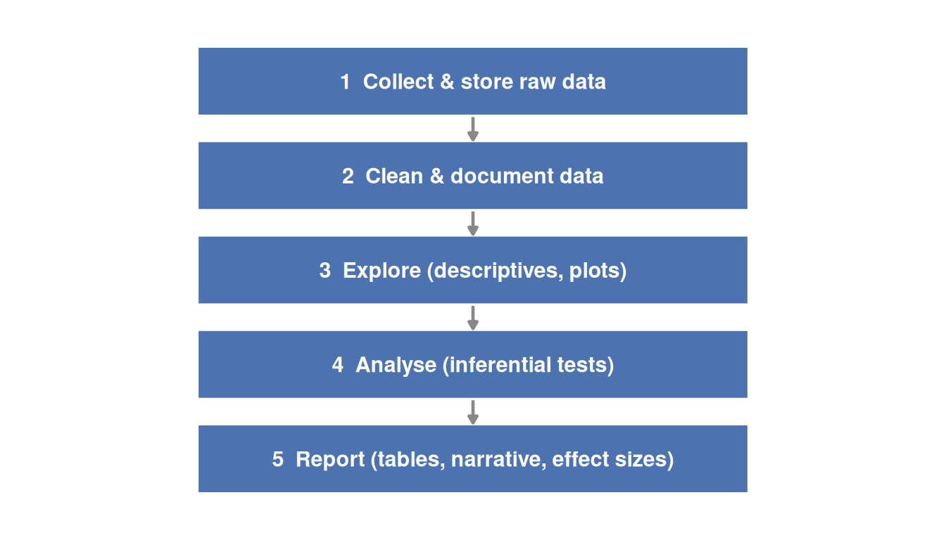
21.7 From Output to Manuscript: A Workflow Overview

A typical analysis workflow moves through five stages, regardless of software:

Figure 21.1: A five-stage analysis workflow. Raw data enter at the top; a reproducible, well-reported manuscript exits at the bottom.

The workflow is the same whether you are using SPSS or R: import data, clean it, explore it, analyse it, and report it. The difference is in how each step is documented. In SPSS, documentation comes from saving syntax files and annotating the output. In R, documentation lives in the script itself.

21.8 Software and the SPSS Appendices in This Book

Throughout this textbook, inferential analyses are illustrated with two parallel tracks:

In-chapter R code — embedded code blocks produce the figures and verify the statistics. These blocks use library(ggplot2) and library(dplyr) and are set to code-fold: true so they do not clutter the reading experience.
SPSS appendix tutorials — step-by-step menu instructions replicate every key analysis for students working in SPSS. Each appendix chapter maps directly to the corresponding textbook chapter.

Either track is sufficient to complete the analyses. Students who become comfortable with both — understanding the logic from the in-chapter discussion, running the procedure in SPSS, and reading the code to see how results were produced — will be well prepared for the diverse software environments of professional practice.

21.9 Decision Guide

Table 21.2 summarizes when to reach for each tool in common movement science scenarios.

Table 21.2: Software selection guide for common movement science research scenarios.

Scenario	Recommended tool
Class assignment, thesis, clinical project	SPSS (with syntax saved)
Replicating a published analysis exactly	R (scripted)
Learning statistics without programming	Jamovi
Bayesian analysis required	JASP
Large dataset, signal processing, ML	Python
Quick descriptive table for a report	Excel
Collaborative manuscript with co-authors using different tools	R + Quarto (renders to any format)

21.10 Practice: quick checks

Every decision is recorded in the script, making the analysis fully reproducible. Anyone with the script and data can re-run all steps exactly as originally performed.

Excel’s statistical functions have documented errors for some procedures and its output is difficult to reproduce systematically. For inferential statistics, a dedicated tool (SPSS, Jamovi, R) is strongly preferred.

Save the SPSS syntax file (.sps). Every menu-driven procedure produces corresponding syntax in the output — copy this to a syntax file after each session. The syntax records every option you selected and can be re-run to reproduce the output exactly.

If the raw file is modified, the original data are lost. All transformations, recoding, and cleaning should be performed by a script or syntax file that reads the raw file and produces a processed version. This preserves the audit trail and allows starting over from scratch if an error is discovered.

Yes — Jamovi is built on R and reads standard .csv data files, as does R. The underlying computations use R packages. Results from Jamovi and R should match for all standard analyses. Sharing cleaned .csv data allows both users to work from the same file; the difference is only in how the interface presents the analysis.

When Bayesian hypothesis testing is a primary goal. JASP is designed to present Bayes Factors alongside frequentist results in a clean interface. R can also compute Bayes Factors (via the BayesFactor package), but JASP makes this accessible without programming.

Read further

^[1] is the canonical citation for R; include it in any manuscript that used R for analysis.^[3] remains the definitive APA task force report on statistical methods in psychology journals and sets out minimum reporting standards that are equally applicable in movement science. For a thorough introduction to the tidyverse approach to data science in R, see^[2].

Next chapter

Chapter 22 moves from how to run analyses to how to report them. You will learn APA style conventions for statistics, what information must accompany every test result, and how to avoid the most common reporting errors in movement science research.