A Note on By-Hand Calculations: The purpose of this book is not to teach tedious by-hand statistical calculations. Modern researchers run these analyses using major software packages. While we provide the underlying equations for conceptual understanding, we strongly recommend relying on software for computation to avoid errors and save time.
Please direct your attention to the SPSS Tutorial: Repeated Measures ANOVA in the appendix for step-by-step instructions on running the analysis, checking the sphericity assumption, applying corrections, computing effect sizes, and interpreting output!
15.1 Chapter roadmap
Movement Science research is saturated with designs in which the same participants are measured more than once — before and after a training program, at weekly intervals across a learning curve, or under several experimental conditions in a single session. A physical therapist might track pain scores at baseline, four weeks, and eight weeks following a rehabilitation protocol. An exercise scientist might measure VO₂max, strength, and sprint speed before, midway through, and after a 12-week conditioning program. A motor learning researcher might record movement error across five practice blocks. In all of these situations, the research question centers on change over time or across conditions within the same individuals, and the statistical challenge is to model that change efficiently and honestly[1–3].
The one-way repeated measures ANOVA is the natural extension of the paired t-test to situations involving three or more within-subject conditions or time points. Just as the paired t-test exploits the correlation between pre and post measurements to eliminate individual differences from the error term, repeated measures ANOVA applies the same logic across multiple time points simultaneously — while maintaining control over the familywise error rate. The result is a test that is substantially more powerful than its between-subjects counterpart: the same number of participants provides far more information when each person serves as their own control, because the large variability among individuals is separated from the error used to test the time effect[4,5]. This efficiency is one of the most compelling reasons to use within-subject designs whenever the research question permits.
This chapter introduces the logic, assumptions, and interpretation of one-way repeated measures ANOVA, building directly on the between-subjects ANOVA framework presented in Chapter 14. You will learn about sphericity — the assumption unique to repeated measures designs that has no parallel in between-subjects ANOVA — and how the Greenhouse-Geisser and Huynh-Feldt corrections protect against inflated Type I error when that assumption is violated. You will also learn how to follow up a significant omnibus test with Bonferroni-corrected pairwise comparisons, how to quantify the size of the within-subject effect using partial eta-squared and partial omega-squared, and how to present these results clearly in APA style. Throughout, the examples draw on the core_session.csv dataset that runs through this textbook, keeping the focus on real movement science data rather than abstract numerical illustrations.
15.2 Learning objectives
By the end of this chapter, you will be able to:
Explain why repeated measures designs offer greater statistical power than equivalent between-subjects designs.
Describe how total variance is partitioned in a one-way repeated measures ANOVA, distinguishing between-subjects variance from within-subjects error.
State the sphericity assumption and explain what it means in plain language.
Interpret Mauchly’s test of sphericity and select the appropriate degrees-of-freedom correction (Greenhouse-Geisser or Huynh-Feldt) when needed.
Conduct and interpret Bonferroni-corrected pairwise comparisons following a significant within-subjects effect.
Compute and interpret partial eta-squared (η²_p) and partial omega-squared (ω²_p) as effect size measures for repeated measures ANOVA.
Report a complete one-way repeated measures ANOVA in APA format, including the sphericity correction used.
15.3 Workflow for one-way repeated measures ANOVA
Use this sequence whenever the same participants are measured at three or more time points or conditions:
Restructure data into wide format in SPSS (one row per participant, one column per time point).
Check assumptions — normality of difference scores and sphericity.
Run the repeated measures ANOVA and inspect Mauchly’s test before reading the F-ratio.
Select the appropriate F-row — sphericity assumed, Greenhouse-Geisser, or Huynh-Feldt — based on Mauchly’s result and epsilon.
If F is significant, run Bonferroni-corrected pairwise comparisons.
Calculate effect sizes (η²_p and ω²_p) from the SPSS output.
Interpret and report results in APA format, including the correction used.
15.4 The logic of repeated measures
15.4.1 Within-subject versus between-subject designs
The fundamental distinction between between-subjects and within-subjects designs concerns what varies across conditions and what stays constant. In a between-subjects design (Chapter 14), each participant is exposed to only one level of the independent variable — they are in the endurance group, or the resistance group, or the control group. Any differences among group means therefore reflect both the true effect of the treatment and all the irreducible differences among people: genetics, training history, motivation, sleep, diet, and countless other factors that make human beings vary.
In a within-subjects (repeated measures) design, the same participants appear in all conditions. A participant who tends to score high on any given measure will score high across all time points; one who tends to score low will be consistently low. This consistency means that each person’s own baseline level cancels out when we compare their scores across conditions — their between-person variability is no longer part of the error term. What remains in the error is only the variability in how differently each participant responds to the conditions, which is typically much smaller than the raw variability among individuals[4,5].
This distinction has profound practical consequences. A between-subjects ANOVA comparing three training groups might require n = 50 per group (150 total) to achieve adequate power for a medium effect. An equivalent within-subjects ANOVA testing the same outcome at three time points within the same participants might require only n = 30 — half the participants, half the recruitment cost, and considerably less data collection burden on each individual[6,7]. The trade-off is that within-subjects designs require participants to be available for multiple assessments, introduce the possibility of carryover effects between conditions, and carry the sphericity assumption discussed below.
15.4.2 The power advantage: partitioning out individual differences
To understand why repeated measures designs are more powerful, consider how total variance is partitioned. In a between-subjects one-way ANOVA (Chapter 14), total variability is divided into two sources: variability between groups (the effect of the treatment) and variability within groups (everything else — individual differences plus random error). The F-ratio is formed by dividing the group effect by this combined within-group variance, which includes all the noise from individual differences.
In a repeated measures ANOVA, a third partition is possible because the same individuals appear in every condition:
\(SS_{\text{between subjects}}\) captures the fact that some participants are consistently higher or lower than others across all time points. This is removed from the denominator of the F-ratio entirely.
\(SS_{\text{time}}\) reflects how much means change across the time points — this is the effect we want to test.
\(SS_{\text{error}}\) (sometimes called the interaction of subjects × time) reflects how differently each participant responds to each time point — random fluctuation that cannot be explained by either the average time trend or consistent individual differences.
Because \(SS_{\text{between subjects}}\) is removed from the error term, the denominator of the F-ratio (\(MS_{\text{error}}\)) is much smaller than in a between-subjects design. A smaller denominator produces a larger F for the same numerator, which directly translates into greater statistical power[4].
TipThink of it as controlling for individual baselines
Imagine you are measuring grip strength before, midway through, and after a 12-week training program. Participant A is a competitive athlete who starts at 110 kg and ends at 118 kg. Participant B is sedentary and starts at 60 kg and ends at 67 kg. A between-subjects design would treat these large baseline differences as error. A repeated measures design instead asks: “Relative to each person’s own starting point, how much did they change?” This individual-as-own-control approach removes the enormous between-person baseline variability from the error term, making the training effect much easier to detect[5].
15.5 One-way repeated measures ANOVA in practice
15.5.1 When to use one-way repeated measures ANOVA
One-way repeated measures ANOVA is appropriate when the same participants provide data under three or more conditions or at three or more time points, and when the goal is to test whether the population mean of a continuous outcome variable differs across those conditions[1–3]. The “one-way” designation means there is a single within-subject factor — for example, time (pre, mid, post) or practice session (1, 2, 3, 4, 5). The design requires that every participant contributes exactly one observation at each level of the factor; missing data at any time point complicates the analysis and needs to be addressed before running the ANOVA.
It is important to recognize the connection to simpler tests. When there are only two time points or conditions, the repeated measures ANOVA reduces exactly to a paired t-test — the two approaches give identical results. Moving to three or more conditions requires the ANOVA framework because comparing all pairs separately would inflate the familywise error rate exactly as described in Chapter 14, and because ANOVA’s omnibus test is more powerful than any set of uncorrected pairwise tests[4]. If the outcome variable is ordinal rather than continuous, or if the normality assumption is severely violated with small samples, the nonparametric Friedman’s ANOVA by ranks (Chapter 19) is the appropriate alternative[8].
The population mean is equal at all time points — time has no effect on the dependent variable.
Alternative hypothesis (H₁):
At least one population mean differs from the others across time points.
As in between-subjects ANOVA, a significant omnibus F only tells you that somewhere across the time points there is a meaningful change; post hoc tests are required to identify which specific pairs of time points differ significantly.
15.5.3 Worked example: Strength gains across a 12-week program
The following example uses data from the core_session.csv dataset. Thirty university students enrolled in a 12-week resistance training program had their muscular strength (kg) measured at three time points: before training began (pre), at the six-week midpoint (mid), and at the end of the program (post).
Step 1: State hypotheses
H₀: μ_pre = μ_mid = μ_post (training has no effect on strength over time)
H₁: Strength differs across at least two of the three time points
α = .05
Step 2: Check assumptions
Verify normality of the difference scores between each pair of time points and check for sphericity using Mauchly’s test (see Assumptions section below, and the SPSS Tutorial for detailed steps).
Mauchly’s test indicated that the sphericity assumption was violated, W = .623, χ²(2) = 13.234, p = .001. Because ε_GG = .726, the Greenhouse-Geisser correction was applied. The within-subjects ANOVA then revealed a significant effect of time:
Source
SS
df
MS
F
p
η²_p
Time
443.73
1.452
305.60
116.0
< .001
.80
Error (Time)
110.94
42.11
2.63
Participants
13,120.63
29
With F(1.45, 42.11) = 116.0, p < .001, η²_p = .80, the effect of training time on muscular strength was large and statistically significant. Post hoc Bonferroni-corrected pairwise comparisons revealed that strength increased significantly from pre to mid (mean difference = 2.0 kg, p < .001), from mid to post (mean difference = 3.4 kg, p < .001), and from pre to post (mean difference = 5.4 kg, p < .001).
NoteReal example: Tracking strength across a training program
Studies examining periodized resistance training routinely use repeated measures ANOVA to quantify how muscular strength, power output, or hypertrophy evolves over a program[2,3]. The within-subjects design is ideal here because inter-individual variability in baseline strength is large — accounting for it substantially increases the sensitivity to detect genuine training-induced change.
15.6 Assumptions of one-way repeated measures ANOVA
Repeated measures ANOVA rests on three assumptions, the last of which is unique to within-subjects designs and absent from between-subjects ANOVA[4,5,9]:
Independence of participants is the first assumption: different participants’ scores must be independent of one another. Note carefully that scores within the same participant are expected to be correlated — that is the whole point of the design. What must be independent is whether one participant’s response to treatment influences another’s. This is ensured by the research design (e.g., random assignment, no contamination across participants) and cannot be corrected statistically if violated.
Normality of difference scores is the second assumption. Unlike between-subjects ANOVA, which requires normality of the raw scores within each group, repeated measures ANOVA requires that the differences between each pair of time points are approximately normally distributed. For the three-time-point case, this means checking that (mid − pre), (post − pre), and (post − mid) each follow an approximately normal distribution[5]. In practice, this assumption is assessed using histograms, Q-Q plots, and Shapiro-Wilk tests on the difference scores. The test is reasonably robust to mild departures when n ≥ 30[10].
Sphericity is the third and most distinctive assumption of repeated measures ANOVA. It has no counterpart in between-subjects designs and is frequently violated in practice, making it the most important assumption to understand and check carefully.
15.6.1 The sphericity assumption
Sphericity requires that the variances of the differences between all pairs of time points are approximately equal[4,11]. For a design with three time points (pre, mid, post), sphericity requires:
Put plainly: the consistency of each participant’s change should be similar across all pairs of time points. If some time intervals produce highly variable changes (some participants improve a lot, others barely at all) while other intervals produce very uniform changes (everyone improves about the same amount), sphericity is violated.
Sphericity matters because the standard repeated measures F-test assumes homogeneous pairwise difference variances when computing its degrees of freedom. When sphericity is violated, the degrees of freedom are too large — the test uses more degrees of freedom than are justified by the data — causing it to be anticonservative: it rejects H₀ more often than the stated α level, inflating Type I error[4,12].
ImportantSphericity is about the differences, not the raw scores
A common misconception is that sphericity requires equal variances of the raw outcome scores across time points (like homogeneity of variance in between-subjects ANOVA). It does not. Sphericity specifically concerns the variances of the pairwise differences. A dataset can have quite different SDs at pre, mid, and post and still meet the sphericity assumption if the changes are consistent across individuals and time pairs[5].
15.6.2 Mauchly’s test of sphericity
Sphericity is formally evaluated with Mauchly’s W[11]. SPSS automatically produces this test whenever you run a repeated measures ANOVA. Mauchly’s W ranges from 0 to 1: a value of 1 indicates perfect sphericity, while values below 1 indicate departures from sphericity.
Interpreting Mauchly’s test:
If p > .05: the sphericity assumption is not rejected; use the “Sphericity Assumed” row in the SPSS output.
If p < .05: the sphericity assumption is violated; apply a correction to adjust the degrees of freedom.
Along with the W statistic and p-value, SPSS reports two epsilon (ε) estimates, which quantify the degree of sphericity departure. Epsilon ranges from 1/(k − 1) (complete non-sphericity) to 1.0 (perfect sphericity), where k is the number of time points. For three time points, the minimum possible epsilon is .50. An epsilon close to 1.0 means sphericity is nearly met; an epsilon far below 1.0 indicates serious violation.
WarningMauchly’s test can be misleading in small and large samples
Like all significance tests, Mauchly’s test is sensitive to sample size. With very small samples it may fail to detect meaningful violations of sphericity; with large samples it may flag trivial departures as significant. Always inspect the epsilon values alongside the p-value — an epsilon ≥ .90 suggests the sphericity assumption is approximately met even if Mauchly’s test is technically significant in a large sample[5,9].
15.7 Corrections for sphericity violations
When Mauchly’s test is significant (or when epsilon is notably below 1.0), the degrees of freedom of the F-test must be corrected downward to restore the proper Type I error rate. SPSS provides three corrected rows in its Within-Subjects Effects output: Greenhouse-Geisser, Huynh-Feldt, and Lower-bound. The choice between the first two is the key decision.
15.7.1 Greenhouse-Geisser correction
The Greenhouse-Geisser (GG) correction multiplies both the numerator and denominator degrees of freedom by the GG epsilon estimate (\(\hat{\varepsilon}_{GG}\)), reducing them from their uncorrected values[12]:
For example, in a three-time-point design with the uncorrected df = 2 for time and df = 58 for error, a GG epsilon of .78 would give corrected df of 1.56 and 45.24, respectively. The F-statistic itself does not change — only the degrees of freedom change, which alters the critical value and p-value. The GG correction is conservative: it tends to overcorrect, especially when epsilon is above .75, which can reduce power unnecessarily[13].
15.7.2 Huynh-Feldt correction
The Huynh-Feldt (HF) correction applies a less conservative epsilon estimate (\(\tilde{\varepsilon}_{HF}\)), which adjusts for the downward bias in the GG estimate[13]. The HF epsilon is always at least as large as the GG epsilon (sometimes considerably larger), resulting in larger corrected degrees of freedom and a more powerful test. When epsilon is high (close to 1.0), the HF-corrected results closely approximate the sphericity-assumed results.
15.7.3 Choosing between the corrections
The widely used decision rule is based on the GG epsilon estimate[5,9]:
If \(\hat{\varepsilon}_{GG} \geq .75\): use the Huynh-Feldt correction — GG is overly conservative here, and HF provides a better balance of Type I error control and power.
If \(\hat{\varepsilon}_{GG} < .75\): use the Greenhouse-Geisser correction — the violation is serious enough that GG’s conservative correction is warranted.
If sphericity is not violated (Mauchly’s p > .05): use the Sphericity Assumed row.
Always report which correction was used and the epsilon value, so readers can evaluate the decision.
TipWhen to skip the correction altogether
If your design has only two levels (e.g., pre and post), sphericity cannot be violated — a two-level within-subjects factor automatically satisfies the assumption. You will see Mauchly’s test grayed out or absent in SPSS output in this case. The repeated measures ANOVA with two levels is equivalent to the paired t-test, and no correction is needed[4].
15.8 Post hoc tests for repeated measures
When the omnibus F is significant, post hoc tests identify which specific pairs of time points differ. The recommended approach in repeated measures designs is Bonferroni-corrected pairwise comparisons, which adjust the significance threshold for the number of comparisons being made[5]. For three time points, there are three possible pairs: pre vs. mid, pre vs. post, and mid vs. post.
SPSS produces Bonferroni-corrected pairwise comparisons automatically when you request estimated marginal means with the Bonferroni adjustment under Options in the Repeated Measures dialog. Each pairwise comparison is reported as a mean difference, its standard error, an adjusted p-value, and a 95% confidence interval. This allows you to determine not only whether each pair differs significantly, but also the magnitude and direction of the difference.
For the strength example, Bonferroni-corrected pairwise comparisons yielded:
Comparison
Mean Difference (kg)
SE
p (adjusted)
95% CI
Mid − Pre
2.02
0.27
< .001
[1.34, 2.70]
Post − Pre
5.38
0.33
< .001
[4.54, 6.22]
Post − Mid
3.36
0.45
< .001
[2.22, 4.50]
All three pairwise comparisons were significant, indicating that strength increased progressively and significantly at each stage of the training program.
ImportantOnly run post hoc tests after a significant omnibus F
The same rule applies here as in between-subjects ANOVA: post hoc pairwise comparisons are only appropriate after a significant omnibus within-subjects F-test. Running comparisons following a non-significant overall result inflates Type I error[4,5].
15.9 Effect sizes for repeated measures ANOVA
15.9.1 Partial eta-squared (η²_p)
SPSS reports partial eta-squared as the default effect size in repeated measures ANOVA. Unlike the full eta-squared (η²) used in between-subjects ANOVA, the partial version excludes between-subjects variance from the denominator[14]:
Note that \(SS_{\text{between subjects}}\) does not appear in this formula. This is why partial eta-squared in repeated measures designs tends to be larger than the full eta-squared computed from the same data — it captures the time effect relative only to within-subject error, after the enormous between-subjects variability has been removed. The benchmarks proposed by Cohen (1988) are typically applied[6]:
η²_p = .01: Small effect
η²_p = .06: Medium effect
η²_p = .14: Large effect
In the strength training example, η²_p = .80 indicates that 80% of the within-subject (error + time) variance is accounted for by the time effect — a very large effect consistent with the powerful and consistent strength gains observed across all 30 participants.
15.9.2 Partial omega-squared (ω²_p)
Just as η² overestimates the population effect in between-subjects ANOVA, η²_p overestimates it in repeated measures ANOVA, particularly with small samples. Partial omega-squared provides a less biased estimate[14,15]:
where \(k\) is the number of time points and \(n\) is the number of participants. SPSS does not compute ω²_p directly, but it can be calculated from the source table values. For the strength example:
This confirms that the time effect is genuinely large, even after correcting for the upward bias in η²_p.
15.9.3 Cohen’s d for pairwise comparisons
For each Bonferroni-corrected pairwise comparison, a Cohen’s d can be computed to quantify the effect size of that specific contrast. For within-subject comparisons, Cohen’s d is computed from the mean difference and the standard deviation of the difference scores:
\[
d = \frac{\bar{D}}{SD_D}
\]
where \(\bar{D}\) is the mean of the difference scores and \(SD_D\) is their standard deviation. Using the real data:
Mid vs. Pre: d = 2.02 / 1.46 = 1.38 (large)
Post vs. Pre: d = 5.38 / 1.81 = 2.97 (very large)
Post vs. Mid: d = 3.36 / 2.47 = 1.36 (large)
These large effect sizes are consistent with what the data show: training-induced strength gains that are consistent across participants, producing tight distributions of difference scores and therefore large standardized effects.
15.10 Visualizing repeated measures results
15.10.1 Line plot with error bars
Code
library(ggplot2)library(dplyr)set.seed(42)# Simulate data matching core_session.csv training group valuesn <-30pre <-rnorm(n, mean =79.7, sd =12.3)mid <- pre +rnorm(n, mean =2.0, sd =1.5)post <- pre +rnorm(n, mean =5.4, sd =1.8)df_long <-data.frame(id =rep(1:n, 3),time =factor(rep(c("Pre", "Mid (6-wk)", "Post (12-wk)"),each = n),levels =c("Pre", "Mid (6-wk)", "Post (12-wk)")),strength =c(pre, mid, post))summary_df <- df_long %>%group_by(time) %>%summarise(M =mean(strength),SD =sd(strength),n =n(),SE = SD /sqrt(n),CI_lo = M -qt(0.975, df = n -1) * SE,CI_hi = M +qt(0.975, df = n -1) * SE )ggplot(summary_df, aes(x = time, y = M, group =1)) +geom_ribbon(aes(ymin = CI_lo, ymax = CI_hi), alpha =0.15, fill ="#5bc0de") +geom_line(linewidth =1.1, colour ="#2c7bb6") +geom_point(size =4, colour ="#2c7bb6") +geom_errorbar(aes(ymin = CI_lo, ymax = CI_hi),width =0.15, linewidth =0.8, colour ="#2c7bb6") +labs(x ="Time Point", y ="Muscular Strength (kg)",title ="Strength Gains Across 12-Week Training Program") +coord_cartesian(ylim =c(65, 100)) +theme_minimal(base_size =13)
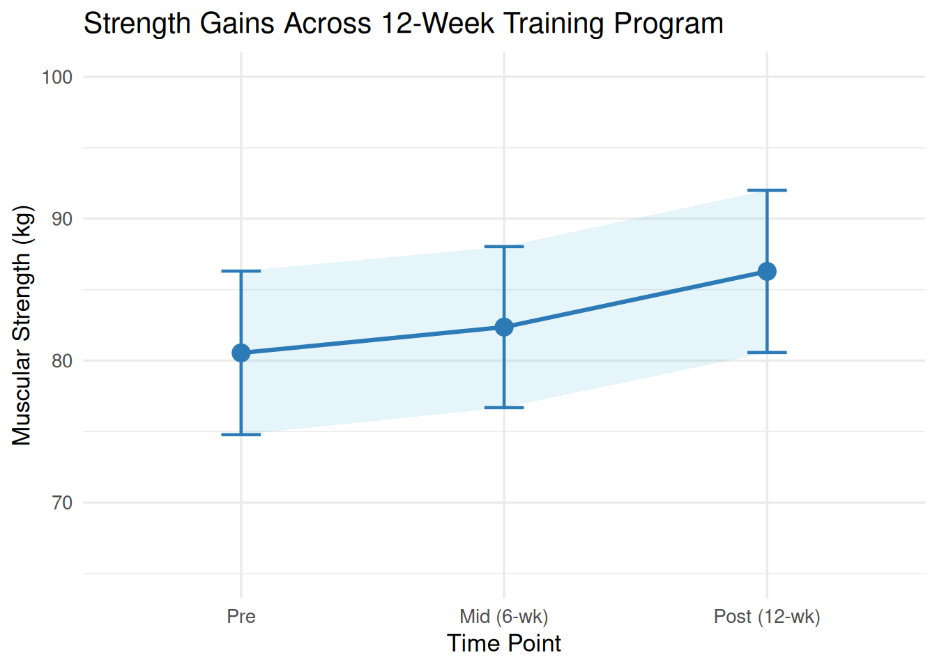
Figure 15.1: Mean muscular strength (kg) with 95% confidence intervals across three training time points (n = 30). Progressive increases from pre- to mid- to post-training are evident, with non-overlapping confidence intervals between pre and post indicating a statistically significant and practically meaningful change.
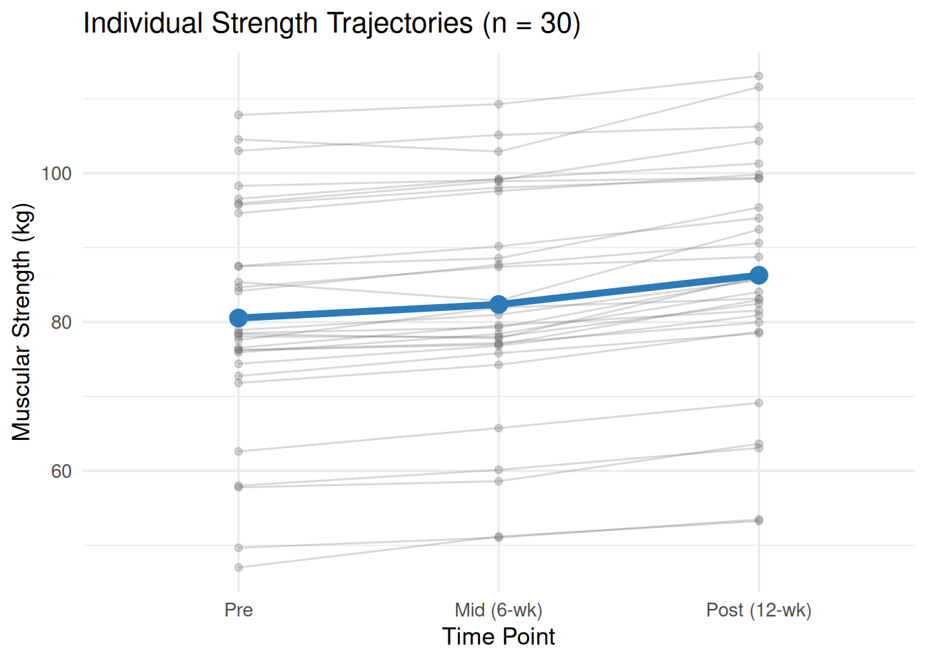
Figure 15.2: Individual participant strength trajectories (spaghetti plot) across three time points. Each thin grey line represents one participant, with the bold blue line showing the group mean. The consistent upward trajectory across virtually all participants illustrates why the within-subjects effect is so large: the training effect is reliable and similar across individuals.
The spaghetti plot (Figure 15.2) is a particularly valuable visualization for repeated measures data because it makes the within-person pattern visible. When lines move predominantly in the same direction — as they do here — the within-subject effect is consistent and the error term will be small, yielding high power. Lines that cross or reverse direction across time points signal inconsistency across participants, larger error variance, and potentially lower power[16,17].
15.11 Reporting repeated measures ANOVA in APA style
A complete APA-style write-up integrates the Mauchly’s test result, the correction applied (if any), the omnibus F, the post hoc comparisons, and the effect size[17,18].
Template:
“A one-way repeated measures ANOVA examined the effect of [factor] on [DV]. Mauchly’s test indicated that the sphericity assumption [was/was not] violated, W([df]) = [W], p = [p]. [Therefore, degrees of freedom were corrected using the [Greenhouse-Geisser/Huynh-Feldt] estimate of sphericity (ε = [value]).] The within-subjects effect of [factor] was [significant/not significant], F([df_time], [df_error]) = [F], p = [p], η²_p = [value]. Post hoc Bonferroni comparisons revealed that [specific pairwise results].”
Full example from the strength training data:
“A one-way repeated measures ANOVA was conducted to examine the effect of training time (pre, mid, post) on muscular strength. Mauchly’s test indicated that the sphericity assumption was violated, W = .623, χ²(2) = 13.234, p = .001. Because ε_GG = .726, the Greenhouse-Geisser correction was applied. The within-subjects effect of time was statistically significant, F(1.45, 42.11) = 116.0, p < .001, η²_p = .80, ω²_p = .88. Post hoc Bonferroni-corrected pairwise comparisons indicated that strength increased significantly from pre-training (M = 79.7, SD = 12.3 kg) to mid-training at six weeks (M = 81.7, SD = 12.3 kg), mean difference = 2.02 kg, p < .001, 95% CI [1.34, 2.70]; from mid-training to post-training at twelve weeks (M = 85.1, SD = 12.5 kg), mean difference = 3.36 kg, p < .001, 95% CI [2.22, 4.50]; and from pre- to post-training, mean difference = 5.38 kg, p < .001, 95% CI [4.54, 6.22].”
TipAlways report which correction was used — and why
Readers cannot evaluate your results without knowing whether you applied the sphericity-assumed F, the GG-corrected F, or the HF-corrected F. Report Mauchly’s test results, the epsilon used, and name the correction. This allows others to assess whether your analytic decisions were appropriate and to compare your results with other studies[9,18].
15.12 Sample size and power for repeated measures ANOVA
Planning sample size for a repeated measures ANOVA requires specifying not only the expected effect size and desired power, but also the correlation among repeated measurements — a parameter unique to within-subjects designs[4,7]. When repeated observations are highly correlated (e.g., participants maintain their relative ordering across time points), the within-subjects design removes more between-subjects variance, the error term shrinks more dramatically, and fewer participants are needed. Conversely, when correlation is low (participants’ scores fluctuate considerably in their relative rank across time points), the efficiency advantage over a between-subjects design diminishes.
In G*Power, power analysis for a one-way repeated measures ANOVA is conducted under F tests → ANOVA: Repeated measures, within factors. You specify the effect size Cohen’s f, α, desired power, the number of groups (1 for a purely within-subject design), the number of measurements (3 for pre/mid/post), and the correlation among repeated measures. Using a medium effect (f = .25), α = .05, power = .80, 3 time points, and a moderate correlation of r = .50, G*Power indicates approximately 28 participants are sufficient — far fewer than the 52 required by an equivalent between-subjects ANOVA[6,7]. The critical practical lesson is that the correlation input matters enormously: higher assumed correlations yield smaller required sample sizes. When in doubt, use a conservative (lower) correlation estimate from pilot data or prior literature.
For those building intuition before running a formal analysis, the Statistical Calculators appendix includes a power calculator supporting t-tests and ANOVA. While it does not yet support the full repeated measures power model, it provides a useful starting point for exploring how effect size and sample size interact.
TipG*Power and SPSS 31 for repeated measures power
G*Power handles repeated measures power analysis with full flexibility over the number of measurements and assumed correlations[7]. SPSS Statistics 31+ also includes a dedicated Analyze → Power Analysis module that covers repeated measures designs. Both tools report the required sample size and allow sensitivity analyses — exploring what effect sizes your planned study can detect at a given N. Using both, as a cross-check, is good practice.
15.13 Common pitfalls and best practices
15.13.1 Pitfall 1: Ignoring Mauchly’s test and always using “Sphericity Assumed”
When Mauchly’s test is significant and epsilon is notably below 1.0, the sphericity-assumed F-test rejects H₀ too often. Routinely using the sphericity-assumed row without checking Mauchly’s test can produce misleading conclusions. Always inspect Mauchly’s result first and apply the appropriate correction — GG or HF — when warranted[12,13].
15.13.2 Pitfall 2: Treating partial eta-squared as though it were full eta-squared
Partial eta-squared (η²_p) reported by SPSS for repeated measures ANOVA excludes between-subjects variance from the denominator, making it larger than the full eta-squared computed from the same data. Reporting η²_p without qualification, or comparing it directly to η² values from between-subjects studies, overstates the proportion of total variance explained. Always clarify that you are reporting partial eta-squared, and consider also reporting ω²_p for a less biased estimate[14,15].
15.13.3 Pitfall 3: Running post hoc tests after a non-significant omnibus F
The same rule applies in repeated measures ANOVA as in between-subjects ANOVA: pairwise comparisons are only justified following a significant omnibus within-subjects F-test. Running them after a non-significant result — perhaps hoping that some individual pairs will be significant even though the overall test is not — inflates Type I error and produces unreliable conclusions[4,5].
15.13.4 Pitfall 4: Confusing within-subjects error with between-subjects variance
The error term in a repeated measures ANOVA (\(MS_{\text{error}}\), sometimes labeled \(MS_{\text{residual}}\) or \(MS_{\text{subjects} \times \text{time}}\)) is not the same as the within-groups error in a between-subjects ANOVA. In repeated measures designs, the F-ratio is computed as \(MS_{\text{time}} / MS_{\text{error}}\), where \(MS_{\text{error}}\) reflects individual inconsistency in responses across time points — not total within-group variability. Understanding this distinction is essential for correctly interpreting the source table SPSS produces[4,9].
15.14 Chapter summary
Repeated measures designs are among the most powerful and efficient research approaches in Movement Science because they exploit the correlation among measurements taken on the same individuals across time or conditions[3,4]. By removing between-subjects variability from the error term, repeated measures ANOVA achieves the same statistical power as a between-subjects ANOVA with substantially fewer participants — an advantage that is especially valuable in clinical and sport science research where participant recruitment is time-consuming and expensive[1,2]. The one-way repeated measures ANOVA extends the paired t-test to three or more time points while maintaining the stated familywise error rate, making it the appropriate choice whenever the same participants contribute continuous outcome data across multiple conditions.
The central technical challenge in repeated measures ANOVA is the sphericity assumption[11]. Unlike between-subjects designs — which require homogeneity of variance across groups — repeated measures designs require that the variances of all pairwise difference scores are approximately equal. Violations of sphericity inflate the Type I error rate of the standard F-test. Mauchly’s test detects such violations, and the epsilon statistic quantifies their severity. When epsilon is below .75, the Greenhouse-Geisser correction provides a conservative but reliable fix; when epsilon is .75 or above, the Huynh-Feldt correction offers a better balance of error control and power[9,12,13]. Following a significant omnibus test, Bonferroni-corrected pairwise comparisons identify which specific time points differ while controlling the familywise error rate.
Effect size reporting in repeated measures ANOVA requires attention to the distinction between partial and full effect sizes. SPSS reports partial eta-squared (η²_p), which excludes between-subjects variance from the denominator; it is typically larger than full η² and should be labeled clearly as partial[14,15]. Partial omega-squared (ω²_p) corrects for the upward bias in η²_p and is recommended for reporting in small-to-moderate samples. For individual pairwise comparisons, Cohen’s d computed from the difference scores quantifies the effect of each specific contrast[6]. Chapter 16 will extend these principles to factorial designs in which two or more factors — at least one of which may be within-subjects — are studied simultaneously, introducing the critical concept of the interaction effect.
In a repeated measures design, each participant provides data at every level of the within-subjects factor, allowing individual baseline differences to be separated out and removed from the error term. Because individual-to-individual variability in movement science outcomes (baseline strength, aerobic capacity, movement speed) is typically large, removing it from the denominator of the F-ratio produces a much smaller error term and a correspondingly larger F. A between-subjects design, by contrast, leaves all individual differences in the error term, reducing the signal-to-noise ratio and requiring more participants to achieve the same power[4,6]. The efficiency gain depends on how strongly correlated the repeated measurements are — the higher the correlation, the greater the advantage of the within-subjects design.
Sphericity requires that the variances of the differences between all pairs of time points are approximately equal[11]. A violation means that some pairwise comparisons show much more variable individual changes than others — for instance, the changes from pre to post may be very inconsistent across participants (some improve greatly, others not at all), while changes from pre to mid are very consistent. When this occurs, the standard repeated measures F-test uses degrees of freedom that are too large, making the test anticonservative: it rejects the null hypothesis more often than the stated α level, inflating Type I error[12]. In practical terms, a violation of sphericity with no correction could lead you to conclude that time has a significant effect when in reality the pattern is unreliable.
Because Mauchly’s test is significant (p = .019), the sphericity assumption has been violated and you should not use the “Sphericity Assumed” row. The next step is to check the GG epsilon: ε_GG = .82, which is greater than .75. Following the decision rule, you should apply the Huynh-Feldt correction rather than the more conservative Greenhouse-Geisser correction[9,13]. Report the HF-corrected F, degrees of freedom, and p-value, and include the epsilon value and the correction name in your APA write-up so readers can evaluate your decision. Note that the F-statistic itself does not change — only the degrees of freedom and the resulting p-value are adjusted.
Full eta-squared (η²) divides \(SS_{\text{time}}\) by the total sum of squares, which includes between-subjects variance (\(SS_{\text{between subjects}}\)). Partial eta-squared (η²_p) divides \(SS_{\text{time}}\) by the sum of \(SS_{\text{time}}\) and \(SS_{\text{error}}\) only — excluding the often-enormous between-subjects component from the denominator[14]. Because between-subjects variance can be very large in human performance data, η²_p is typically considerably larger than full η² computed from the same numbers. This is not an error — it is the intended behavior of a partial effect size, which asks “how large is the time effect relative to the within-person error?” rather than “how large is the time effect relative to everything?”. When comparing effect sizes across studies or designs, always check whether the reported η² is partial or full[15].
With p = .130 > α = .05, the within-subjects effect of time is not statistically significant. The researcher should conclude that the evidence is insufficient to support a change in balance error scores over time — but they should not conclude that time had no effect[19,20]. An important next step is to compute and report partial eta-squared and its confidence interval. If η²_p is modest (e.g., .10) but the confidence interval is wide, the study was likely underpowered to detect a clinically meaningful change, and a larger sample or longer intervention period would be informative. Post hoc pairwise comparisons should not be run following a non-significant omnibus F, as doing so capitalizes on chance[5]. The researcher should also verify that all assumptions were checked and that the appropriate sphericity correction was applied.
A complete APA-style report should include: (1) Mauchly’s test — W, df, p-value — to demonstrate that sphericity was evaluated; (2) the correction applied and the epsilon value, if sphericity was violated; (3) the omnibus F-statistic with corrected degrees of freedom, exact p-value, and at least one effect size (η²_p is required; ω²_p is recommended for small samples); (4) descriptive statistics for each time point (M and SD); and (5) Bonferroni-corrected pairwise comparisons for each significant or theoretically meaningful pair, including mean differences, standard errors, adjusted p-values, and 95% confidence intervals[17,18,21]. Omitting any of these elements leaves readers unable to evaluate the analysis, replicate the findings, or use the results in a meta-analysis.
NoteRead further
For thorough coverage of repeated measures designs, see Maxwell, Delaney & Kelley (2018)[4] (Designing Experiments and Analyzing Data) and Girden (1992)[9] (ANOVA: Repeated Measures). For the original sphericity papers, consult Mauchly (1940)[11], Greenhouse and Geisser (1959)[12], and Huynh and Feldt (1976)[13]. For SPSS-based guidance, Field (2018)[5] provides comprehensive step-by-step instructions. For Movement Science applications, see Vincent (2005)[3] and Portney & Watkins (2020)[2].
TipNext chapter
Chapter 16 extends the repeated measures framework to factorial ANOVA, in which two or more independent variables — which may be between-subjects, within-subjects, or a mix of both — are studied simultaneously. You will learn how to interpret main effects and interaction effects, why interactions are often the most theoretically interesting findings in factorial designs, and how to decompose and visualize interactions in Movement Science data.
2. Portney, L. G., & Watkins, M. P. (2020). Foundations of clinical research: Applications to practice.
3. Vincent, W. J. (2005). Statistics in kinesiology.
4. Maxwell, S. E., Delaney, H. D., & Kelley, K. (2018). Designing experiments and analyzing data: A model comparison perspective (3rd ed.). Routledge.
5. Field, A. (2018). Discovering statistics using IBM SPSS statistics (5th ed.). SAGE Publications.
6. Cohen, J. (1988). Statistical power analysis for the behavioral sciences (2nd ed.). Lawrence Erlbaum Associates.
7. Faul, F., Erdfelder, E., Lang, A.-G., & Buchner, A. (2007). G*power 3: A flexible statistical power analysis program for the social, behavioral, and biomedical sciences. Behavior Research Methods, 39(2), 175–191. https://doi.org/10.3758/BF03193146
8. Conover, W. J. (1999). Practical nonparametric statistics.
9. Girden, E. R. (1992). ANOVA: Repeated measures. Sage.
10. Blanca, M. J., Alarcón, R., Arnau, J., Bono, R., & Bendayan, R. (2013). Non-normal data: Is ANOVA still a valid option? Psicothema, 25(4), 552–557. https://doi.org/10.7334/psicothema2013.552
11. Mauchly, J. W. (1940). Significance test for sphericity of a normal n-variate distribution. Annals of Mathematical Statistics, 11(2), 204–209. https://doi.org/10.1214/aoms/1177731915
12. Greenhouse, S. W., & Geisser, S. (1959). On methods in the analysis of profile data. Psychometrika, 24(2), 95–112. https://doi.org/10.1007/BF02289823
13. Huynh, H., & Feldt, L. S. (1976). Estimation of the box correction for degrees of freedom from sample data in randomized block and split-plot designs. Journal of Educational Statistics, 1(1), 69–82. https://doi.org/10.3102/10769986001001069
14. Olejnik, S., & Algina, J. (2003). Generalized eta and omega squared statistics: Measures of effect size for some common research designs. Psychological Methods, 8(4), 434–447. https://doi.org/10.1037/1082-989X.8.4.434
15. Lakens, D. (2013). Calculating and reporting effect sizes to facilitate cumulative science: A practical primer for t-tests and ANOVAs. Frontiers in Psychology, 4, 863. https://doi.org/10.3389/fpsyg.2013.00863
16. Cumming, G. (2012). Understanding the new statistics: Effect sizes, confidence intervals, and meta-analysis. Routledge.
17. Wilkinson, L., & Task Force on Statistical Inference. (1999). Statistical methods in psychology journals: Guidelines and explanations. American Psychologist, 54(8), 594–604. https://doi.org/10.1037/0003-066X.54.8.594
18. American Psychological Association. (2020). Publication manual of the american psychological association (7th ed.). American Psychological Association.
19. Altman, D. G., & Bland, J. M. (1995). Statistics notes: Absence of evidence is not evidence of absence. BMJ, 311, 485. https://doi.org/10.1136/bmj.311.7003.485