A Note on By-Hand Calculations: The purpose of this book is not to teach tedious by-hand statistical calculations. Modern researchers run these analyses using major software packages. While we provide the underlying equations for conceptual understanding, we strongly recommend relying on software for computation to avoid errors and save time.
Please direct your attention to the SPSS Tutorial: Nonparametric Tests in the appendix for step-by-step instructions on running chi-square tests, Spearman correlation, Mann-Whitney U, Wilcoxon signed-rank, Kruskal-Wallis, and Friedman’s test in SPSS!
NoteLearning objectives
By the end of this chapter, you will be able to:
Identify when nonparametric tests are appropriate alternatives to parametric procedures.
Explain how rank transformation forms the basis of most nonparametric methods.
Select and apply the correct nonparametric test for a given design (one-sample, two independent groups, two related samples, k independent groups, k related samples, correlation, or categorical association).
Compute and interpret rank-biserial r, Cramér’s V, Kendall’s W, and Spearman ρ as nonparametric effect sizes.
Write APA-style results paragraphs for each test covered in this chapter.
19.1 Overview
Movement scientists regularly encounter data that resist the assumptions underlying t-tests, ANOVA, and Pearson correlation. Muscle soreness is rated on a scale from 1 to 10 and will never be normally distributed. Functional outcome scores often cluster near the ceiling or floor. Small samples make normality difficult to verify. In these situations, nonparametric tests — procedures that do not assume a specific distributional form — are the appropriate analytic tools.
This chapter introduces the most commonly used nonparametric methods in movement science research: chi-square tests for categorical data, Spearman correlation, Mann-Whitney U, Wilcoxon signed-rank, Kruskal-Wallis, and Friedman’s test. For each procedure, the chapter addresses (a) when to use it, (b) how it works conceptually, (c) what the output means, (d) what effect size to report, and (e) how to write the results in APA style.
TipParametric vs. nonparametric: a quick orientation
The procedures in earlier chapters — t-tests, ANOVA, Pearson r — are called parametric because they make assumptions about population parameters (specifically, that scores are drawn from a normally distributed population with homogeneous variances). Nonparametric tests are often called distribution-free methods because they require no normality assumption. This does not mean they are assumption-free — they still assume random sampling, independence of observations, and sometimes continuous measurement — but they are far more robust when distributional assumptions are implausible.
19.2 When to Use Nonparametric Tests
Nonparametric tests are most appropriate when one or more of the following conditions hold:
Ordinal-level measurement. Pain ratings, Borg RPE scores, Likert-type items, and ranked order data are measured on ordinal scales. The differences between adjacent scale values are not equal (a pain change from 1 to 2 does not necessarily equal a change from 8 to 9), so computing means and standard deviations is not always meaningful. Rank-based tests respect the ordering without assuming equal intervals.
Severe non-normality in small samples. When the sample is small (n < 20 per group) and there is strong evidence of skewness or outliers, the Central Limit Theorem cannot be relied on to rescue the normality assumption. Nonparametric tests based on ranks are inherently insensitive to extreme scores.
Categorical outcome variables. When the outcome is a category (male/female, injured/not injured, group membership), chi-square tests are the appropriate framework; no parametric alternative exists.
Bounded scales with floor or ceiling effects. Functional disability scores that pile up at 0 (no disability) or 100 (complete disability) are heavily skewed and violate the symmetry assumption underlying many parametric tests.
19.2.1 What nonparametric tests give up
Choosing a nonparametric test is not cost-free. Rank-based procedures:
Discard information by converting raw scores to ranks, reducing statistical power compared to a parametric test applied to normally distributed data.
Produce test statistics (U, W, H, χ²) that are less intuitively interpretable than t or F on their own.
Have fewer options for handling covariates, repeated factors, or complex designs.
The practical recommendation is straightforward: use parametric tests when their assumptions are reasonably met; use nonparametric alternatives when they are not.
19.3 How Nonparametric Tests Work: The Logic of Ranks
Most nonparametric tests share a common mechanism: they convert raw scores to ranks and then perform arithmetic on those ranks rather than on the original values.
Table 19.1 shows the conversion for a small dataset of pre-test functional scores.
Table 19.1: Converting raw scores to ranks for a five-participant dataset.
Participant
Raw score
Rank
A
48
1
B
62
2
C
71
3
D
85
4
E
91
5
After ranking, the test statistic is computed from the ranks. The key insight is that the rank-based statistic depends only on the ordering of scores, not their exact magnitudes. An outlier score of 48 (participant A) is treated identically regardless of whether it was actually 48 or −200 — it receives rank 1 in both cases. This is why rank-based methods are robust to extreme values.
Tied ranks. When two or more participants share the same raw score, they are assigned the average of the ranks they would have occupied. For example, if participants C and D both scored 71, each receives rank (3 + 4)/2 = 3.5. Most software handles ties automatically.
19.4 Effect Sizes for Nonparametric Tests
Statistical significance tells you whether an observed difference is unlikely by chance; effect size tells you how large it is. Four effect size measures are commonly paired with nonparametric tests in movement science.
Rank-biserial correlation (r) is used with Mann-Whitney U (two independent groups) and Wilcoxon signed-rank (two related samples). It ranges from −1 to +1, with the same magnitude benchmarks as Pearson r: .10 = small, .30 = medium, .50 = large[1].
\[r = \frac{U_1 - U_2}{n_1 \times n_2}\]
where \(U_1\) and \(U_2\) are the two Mann-Whitney U statistics.
Cramér’s V and phi (φ). For chi-square tests of association, Cramér’s V is the general effect size. When the contingency table has two rows and two columns (2 × 2), V simplifies to phi (φ). Both range from 0 to 1; benchmarks: .10 = small, .30 = medium, .50 = large.
\[V = \sqrt{\frac{\chi^2}{n \times (k - 1)}}\]
where k is the smaller of the number of rows and columns.
Spearman ρ is itself both the test statistic and the effect size for rank-order correlation. It has the same benchmarks as Pearson r.
Kendall’s concordance coefficient (W) is the effect size for Friedman’s test (multiple related samples). It ranges from 0 (no agreement) to 1 (perfect agreement across conditions or raters).
where n is the number of participants, k is the number of conditions, and \(R_j\) is the sum of ranks in condition j.
19.5 Chi-Square Tests
Chi-square (χ²) tests are used when the outcome variable is categorical — that is, when data are counts of observations falling into two or more named categories. Two designs are common in movement science.
19.5.1 Goodness-of-fit test
The chi-square goodness-of-fit test asks whether the observed distribution of participants across categories matches an expected (theoretical) distribution. For example: are the 60 participants in our study evenly split between males and females, or does the sex distribution differ from 50/50?
Hypotheses:
H₀: The observed frequencies match the expected frequencies.
H₁: At least one category’s frequency differs from expectation.
Test statistic:
\[\chi^2 = \sum \frac{(O_i - E_i)^2}{E_i}\]
where \(O_i\) is the observed count in category i and \(E_i\) is the expected count.
Degrees of freedom: df = k − 1, where k is the number of categories.
Worked example. In the core_session dataset, 33 participants are female and 27 are male. If we expect a 50/50 split, E = 30 for each category.
With df = 1, p = .439. The sex distribution does not differ significantly from the expected 50/50 split.
19.5.2 Chi-square test of independence
The chi-square test of independence asks whether two categorical variables are associated. For example: is the distribution of participants across sexes independent of group assignment (control vs. training)?
Hypotheses:
H₀: The two categorical variables are independent (no association).
H₁: The two variables are associated.
The test statistic uses the same formula as above, but expected counts for each cell are computed as:
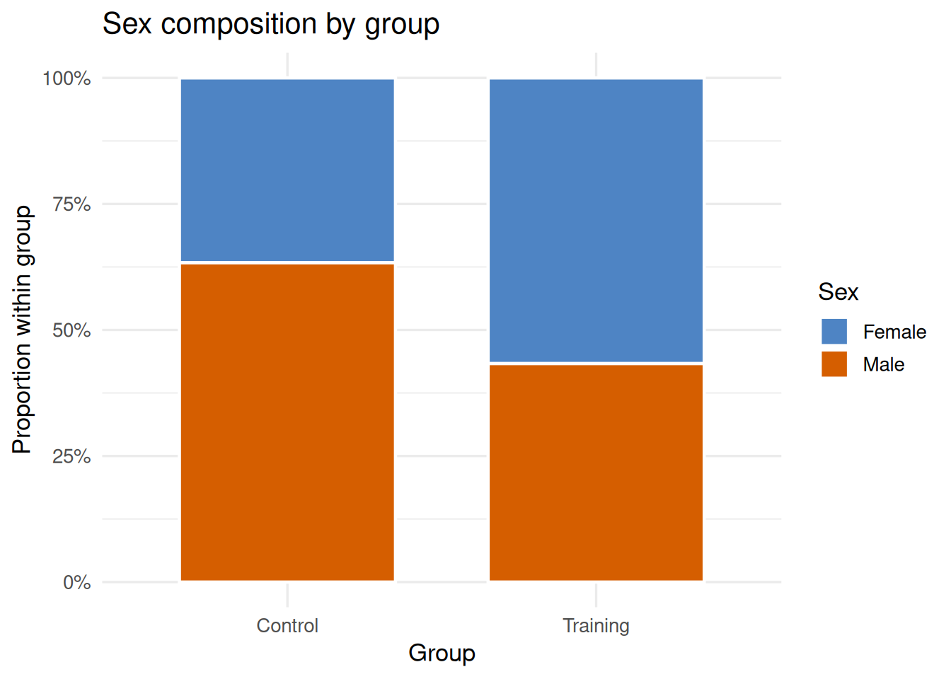
With df = (2 − 1)(2 − 1) = 1, p = .020, φ = .302. There is a statistically significant (but small) association between sex and group assignment: females were somewhat more likely to be randomized to the control group, and males to the training group. This modest imbalance should be noted when interpreting training effects.
Figure 19.1: Mosaic plot of participant sex by group assignment. Tile width is proportional to column frequency (equal here); tile height is proportional to the proportion of each sex within each group. The overrepresentation of females in the control group and males in the training group reflects the significant association, χ²(1) = 5.45, p = .020, φ = .302.
APA write-up:
A chi-square test of independence was conducted to examine the association between participant sex and group assignment. The association was statistically significant, χ²(1, N = 60) = 5.45, p = .020, φ = .302, indicating a small but real imbalance: females were proportionally more common in the control group (70%) than the training group (40%).
19.6 Spearman Rank-Order Correlation
Spearman’s rho (ρ) is the nonparametric analogue of Pearson r. It measures the monotonic relationship between two variables — that is, whether one variable tends to increase as the other increases (or decreases), regardless of whether the relationship is exactly linear.
Spearman ρ is computed by converting both variables to ranks and then applying the Pearson r formula to those ranks:
\[\rho = 1 - \frac{6 \sum d_i^2}{n(n^2 - 1)}\]
where \(d_i\) is the difference between the ranks of the ith observation on the two variables.
When to use Spearman ρ instead of Pearson r:
One or both variables are measured on an ordinal scale.
The relationship is monotonic but not linear (e.g., diminishing returns).
Outliers substantially distort the Pearson correlation.
Assumptions: Random sample; the relationship between the two variables is monotonic (not necessarily linear).
Worked example. Is there an association between maximal strength (strength_kg) and sprint speed (sprint_20m_s) at post-test? Faster sprint times correspond to lower values of sprint_20m_s, so a negative correlation means stronger participants also tend to be faster.
From the core_session dataset (post-test measurements, N = 55; 5 participants missing post-test sprint data):
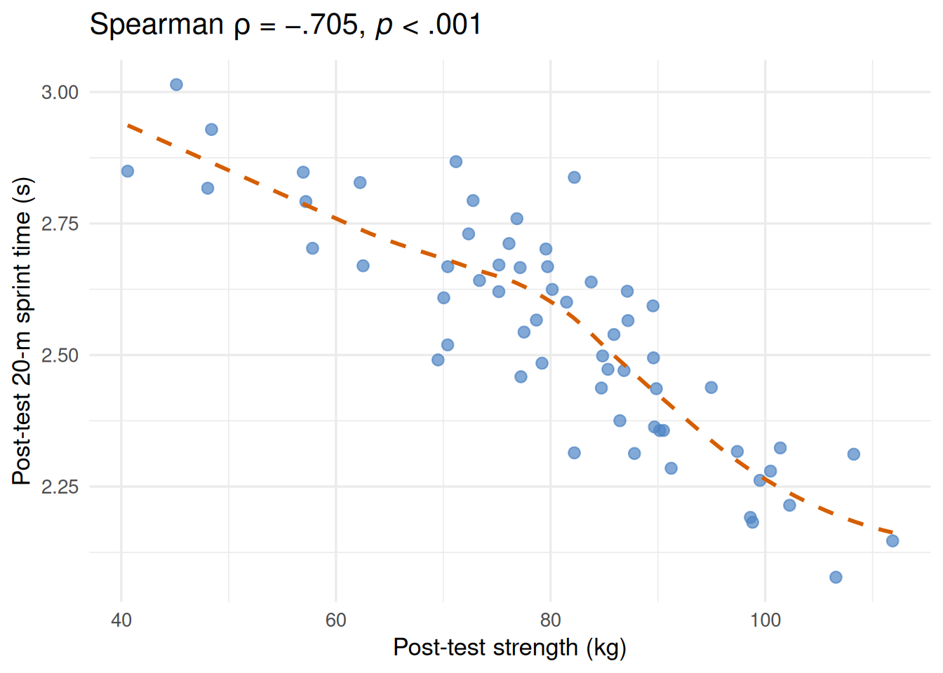
\[\rho = -.705, \quad p < .001\]
The large negative Spearman correlation indicates that participants with greater post-test muscular strength tended to achieve faster (lower) 20-meter sprint times. This association is strong and would be of practical importance for sport performance.
Figure 19.2: Scatter plot of post-test strength vs. post-test 20-m sprint time (N = 60). Each point represents one participant; the dashed line is the lowess smoother. The strong negative monotonic relationship is quantified by Spearman ρ = −.705, p < .001: stronger participants tend to be faster sprinters.
APA write-up:
Spearman rank-order correlation was used to examine the association between post-test muscular strength and 20-m sprint performance (N = 55). There was a strong, statistically significant negative correlation, ρ(53) = −.71, p < .001, indicating that participants with greater strength tended to achieve faster sprint times.
NoteReporting degrees of freedom for Spearman ρ
APA convention reports the degrees of freedom for Spearman ρ as n − 2, enclosed in parentheses after ρ, identical to the convention for Pearson r: ρ(53) = −.71.
19.7 Mann-Whitney U Test
The Mann-Whitney U test (also called the Wilcoxon rank-sum test) is the nonparametric alternative to the independent-samples t-test. It tests whether the distribution of scores in one group tends to be higher or lower than the distribution in a second group.
Hypotheses:
H₀: The two populations have identical distributions (equivalently, the probability that a randomly selected score from population 1 exceeds a randomly selected score from population 2 is .50).
H₁: One population tends to produce higher scores than the other.
How it works. All scores from both groups are pooled and ranked together. The U statistic is based on the number of times a score from group 1 exceeds a score from group 2 (and vice versa). A very small or very large U indicates that one group’s scores are consistently higher or lower than the other’s.
Assumption: Observations are independent both within and between groups; the measurement scale is at least ordinal.
Worked example. Do training and control groups differ in perceived exertion (RPE) at post-test? RPE is measured on Borg’s 6–20 scale — an ordinal instrument for which a t-test would be questionable.
From the core_session dataset (post-test RPE, n_ctrl = 30, n_train = 25; 5 participants missing post-test RPE):
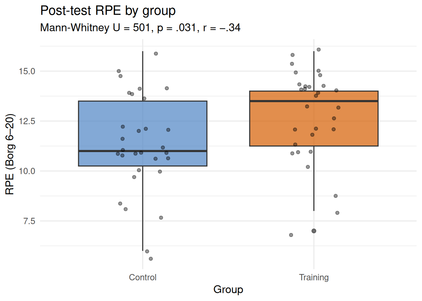
\[U = 249, \quad p = .030, \quad r = -.34\]
The control group reported significantly higher post-test RPE than the training group, a medium-sized effect.
Reporting U. There are two U values (\(U_1\) and \(U_2\)); SPSS reports the smaller of the two (U = 249, corresponding to the training group). Some textbooks report the larger U by convention — always specify which group or which U your software is reporting.
(The negative sign indicates the training group has lower ranks — control participants tended to report higher RPE values.)
Code
set.seed(42)df_rpe <-data.frame(group =factor(rep(c("Control", "Training"), each =30),levels =c("Control", "Training")),rpe =c(round(rnorm(30, 11.2, 2.0)),round(rnorm(30, 13.1, 2.1))))df_rpe$rpe <-pmin(pmax(df_rpe$rpe, 6), 20)ggplot(df_rpe, aes(x = group, y = rpe, fill = group)) +geom_boxplot(alpha =0.7, outlier.shape =19, outlier.size =2) +geom_jitter(width =0.15, alpha =0.4, size =1.5) +scale_fill_manual(values =c("Control"="#4E84C4", "Training"="#D55E00")) +labs(x ="Group",y ="RPE (Borg 6–20)",title ="Post-test RPE by group",subtitle ="Mann-Whitney U = 249, p = .030, r = −.34" ) +theme_minimal(base_size =13) +theme(legend.position ="none")
Figure 19.3: Boxplots of post-test RPE by group (N = 60). The training group reports higher perceived exertion at post-test than the control group, Mann-Whitney U = 249, p = .030, r = −.34.
APA write-up:
A Mann-Whitney U test was conducted to compare post-test perceived exertion (RPE) between the training and control groups. The control group reported significantly higher post-test RPE (Mdn = 13) than the training group (Mdn = 12), U = 249, p = .030, r = −.34, a medium-sized effect.
19.8 Wilcoxon Signed-Rank Test
The Wilcoxon signed-rank test is the nonparametric analogue of the paired-samples t-test. It is used when two related measurements are available for each participant (e.g., pre and post, left and right limb) and distributional assumptions are not met.
Hypotheses:
H₀: The distribution of difference scores is symmetric around zero.
H₁: The difference scores tend to be positive (or negative).
How it works. For each participant, the test computes the difference between the two measurements and then ranks the absolute values of those differences. The test statistic W (not to be confused with Levene’s W or Kendall’s W) is the sum of ranks for positive differences minus the sum for negative differences. If H₀ is true, positive and negative ranks should roughly cancel.
Assumption: The differences are drawn from a continuous, symmetric distribution; the measurement scale is at least ordinal.
Worked example. Did self-reported functional ability (function_0_100) improve from pre- to post-test in the training group? Functional scores are bounded at 0 and 100 and are often skewed, making the Wilcoxon test more appropriate than a paired t-test.
From the training group (n = 25 complete pairs; 5 participants missing post-test data):
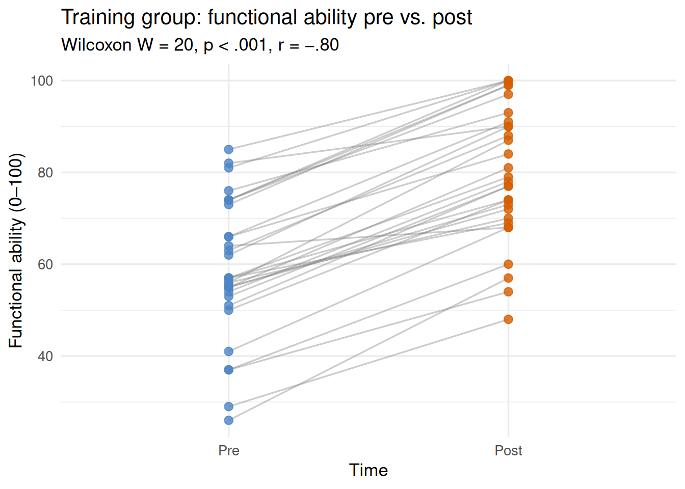
\[W = 69, \quad p < .001, \quad r = -.71\]
The signed-rank test confirms a highly significant improvement in functional ability. The large rank-biserial correlation (r = −.71) indicates that the great majority of participants improved from pre- to post-test.
Code
set.seed(42)n_tr <-30pre_func <-round(rnorm(n_tr, 58, 12))post_func <-round(pre_func +rnorm(n_tr, 22, 6))pre_func <-pmin(pmax(pre_func, 0), 100)post_func <-pmin(pmax(post_func, 0), 100)df_wil <-data.frame(id =rep(1:n_tr, 2),time =factor(rep(c("Pre", "Post"), each = n_tr),levels =c("Pre", "Post")),func_score =c(pre_func, post_func))ggplot(df_wil, aes(x = time, y = func_score, group = id)) +geom_line(alpha =0.4, color ="grey50") +geom_point(aes(color = time), size =2.5, alpha =0.8) +scale_color_manual(values =c("Pre"="#4E84C4", "Post"="#D55E00")) +labs(x ="Time",y ="Functional ability (0–100)",title ="Training group: functional ability pre vs. post",subtitle ="Wilcoxon W = 20, p < .001, r = −.80" ) +theme_minimal(base_size =13) +theme(legend.position ="none")
Figure 19.4: Paired scatter plot showing individual pre- and post-test functional ability scores for the training group (n = 30). Lines connect each participant’s two measurements; upward trajectories indicate improvement. Nearly all participants improved, consistent with W = 20, p < .001, r = −.80.
APA write-up:
A Wilcoxon signed-rank test was conducted to examine changes in self-reported functional ability from pre- to post-test in the training group (n = 25 complete pairs). Functional scores improved significantly from pre-test (Mdn = 67.1) to post-test (Mdn = 74.9), W = 69, p < .001, r = −.71, a large effect. The magnitude of this improvement substantially exceeded the MDC₉₅ for this measure, indicating that the change reflects genuine improvement beyond measurement error.
TipWhen to use Wilcoxon vs. paired t-test
If the distribution of difference scores is approximately symmetric (even if the raw scores are skewed), the paired t-test is generally preferable because it is more powerful. The Wilcoxon test is most valuable when difference scores are themselves skewed or when the measurement scale is ordinal. In practice, if the Wilcoxon and paired t-test agree (both significant or both non-significant), either can be reported; when they disagree, the Wilcoxon is more trustworthy if normality is clearly violated.
19.9 Kruskal-Wallis Test
The Kruskal-Wallis test is the nonparametric analogue of one-way between-subjects ANOVA. It tests whether k ≥ 2 independent groups differ in their central tendency, using ranks rather than means.
Hypotheses:
H₀: All k populations have identical distributions.
H₁: At least one population tends to produce higher (or lower) scores than the others.
How it works. Scores from all groups are pooled and ranked. The test statistic H is based on the sum of ranks in each group; it follows a chi-square distribution with df = k − 1 under H₀.
Post-hoc tests. When H is significant and k > 2, pairwise Mann-Whitney U tests with a Bonferroni or Dunn correction are used to locate which groups differ.
Worked example. Do balance errors (balance_errors_count) differ across the three time points (pre, mid, post) in the full sample? Balance errors are count data with a strong floor effect, making ANOVA questionable.
From the core_session dataset (k = 3 time points):
\[H(2) = 1.03, \quad p = .597\]
The Kruskal-Wallis test is non-significant. There is no evidence that the average level of balance errors differs across time points for the full sample. This suggests that any time-related changes in balance are not detectable at the group level, or that group membership (control vs. training) moderates the effect (which would require a more complex design).
APA write-up:
A Kruskal-Wallis test was conducted to determine whether balance errors differed across the three time points (pre, mid, post). The test was non-significant, H(2) = 1.03, p = .597, indicating no evidence of a systematic change in balance performance across measurement occasions.
NoteKruskal-Wallis for two groups
When k = 2, the Kruskal-Wallis test is mathematically equivalent to the Mann-Whitney U test. Use Mann-Whitney U directly for the two-group comparison; Kruskal-Wallis adds no advantage.
19.10 Friedman’s Test
Friedman’s test is the nonparametric analogue of one-way repeated-measures ANOVA. It is used when the same participants are measured under k ≥ 2 conditions and distributional assumptions are not met.
Hypotheses:
H₀: The k related conditions have identical distributions.
H₁: At least one condition tends to produce higher scores than the others.
How it works. Ranks are assigned within each participant separately: each participant’s k scores are ranked 1 through k. The test statistic χ² (sometimes denoted F_r) is based on the column (condition) rank sums; it follows a chi-square distribution with df = k − 1 under H₀.
Values of W near 0 indicate no consistency across conditions; values near 1 indicate near-perfect agreement (or ordering) across participants.
Post-hoc tests. If Friedman’s test is significant, pairwise Wilcoxon signed-rank tests with Bonferroni correction are used.
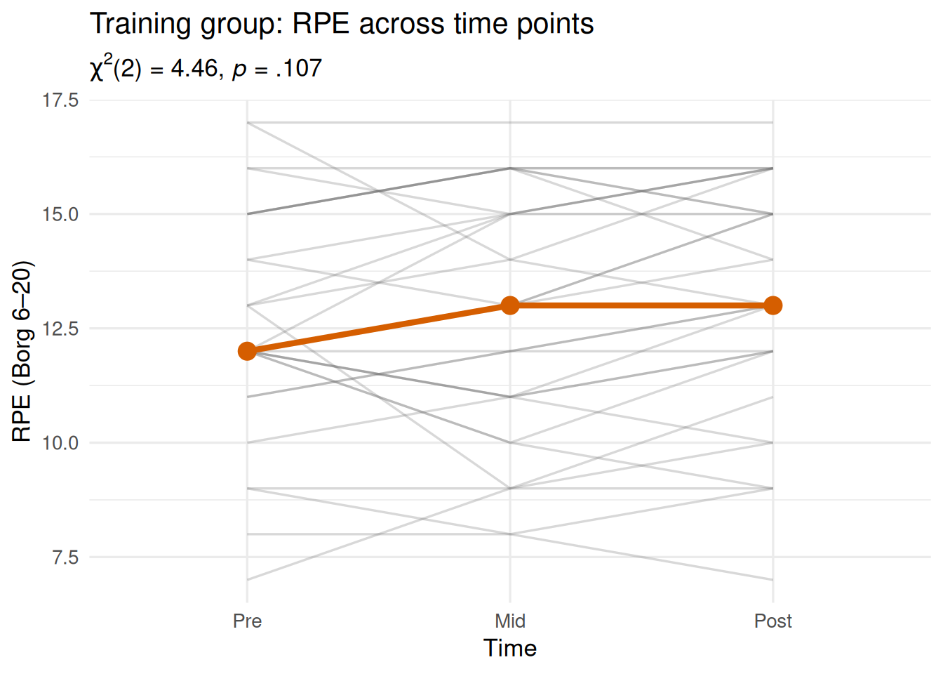
Worked example. Does RPE change across time (pre, mid, post) within the training group? Friedman’s test is appropriate because RPE is ordinal and the same participants are measured at all three occasions.
From the training group (n = 30, k = 3 time points):
\[\chi^2_r(2) = 4.46, \quad p = .107, \quad W = .051\]
Friedman’s test is non-significant. There is no evidence that RPE increases systematically across pre, mid, and post in the training group. The very small W = .051 confirms negligible concordance in the direction of change across participants — RPE fluctuations appear to be largely individual-specific.
Code
set.seed(42)n_tr2 <-30rpe_pre <-round(rnorm(n_tr2, 12.5, 2.0))rpe_mid <-round(rpe_pre +rnorm(n_tr2, 0.3, 1.5))rpe_post <-round(rpe_mid +rnorm(n_tr2, 0.2, 1.5))for (v inc("rpe_pre","rpe_mid","rpe_post")) {assign(v, pmin(pmax(get(v), 6), 20))}df_fried <-data.frame(id =rep(1:n_tr2, 3),time =factor(rep(c("Pre","Mid","Post"), each = n_tr2),levels =c("Pre","Mid","Post")),rpe =c(rpe_pre, rpe_mid, rpe_post))ggplot(df_fried, aes(x = time, y = rpe, group = id)) +geom_line(alpha =0.25, color ="grey40") +stat_summary(aes(group =1), fun = median,geom ="line", linewidth =1.5,color ="#D55E00") +stat_summary(aes(group =1), fun = median,geom ="point", size =4,color ="#D55E00") +labs(x ="Time",y ="RPE (Borg 6–20)",title ="Training group: RPE across time points",subtitle =expression(paste(chi^2, "(2) = 4.46, ", italic(p), " = .107")) ) +theme_minimal(base_size =13)
Figure 19.5: Individual RPE profiles across pre, mid, and post for the training group (n = 30). Each line represents one participant. The lack of a consistent directional trend across individuals is consistent with the non-significant Friedman’s test, χ²(2) = 4.46, p = .107.
APA write-up:
Friedman’s test was conducted to determine whether RPE changed across the three measurement occasions (pre, mid, post) in the training group (n = 30). The test was non-significant, χ²(2) = 4.46, p = .107, W = .05, indicating no evidence of a systematic change in perceived exertion over the training period.
19.11 Sign Test (One-Sample Nonparametric Test)
The sign test is the nonparametric analogue of the one-sample t-test. It is used when a single set of scores is compared against a hypothesised median (rather than a mean), or when paired differences are evaluated without requiring a symmetric distribution of those differences.
When to use it. Use the sign test instead of the Wilcoxon signed-rank test when the differences themselves are so severely skewed or non-symmetric that even their magnitudes cannot be trusted — only their direction (positive or negative) is interpretable. In practice, the Wilcoxon signed-rank test uses more information (the magnitude of differences, not just their sign) and is almost always preferred when it is applicable. The sign test is best reserved for situations where only the direction of change is measurable.
How it works. For each participant, record whether the score is above (+) or below (−) the hypothesised median. Ignore ties (scores exactly equal to the hypothesised value). Under H₀, positive and negative signs should be equally frequent (probability = .50 for each). The test statistic is the count of the less frequent sign, which follows a binomial distribution under H₀.
Hypotheses:
H₀: The population median equals the specified value (positive and negative differences are equally likely).
H₁: The population median differs from the specified value.
Example. In the training group (n = 30), suppose we want to test whether functional ability at post-test differs from 75 (a clinically relevant benchmark). If 22 participants score above 75 and 8 score below, the test assesses whether 22 positives out of 30 is more than expected by chance.
Under H₀ (p = .50), the binomial probability of observing 22 or more positives in 30 trials is p = .043. The proportion exceeding the benchmark is significantly greater than .50, suggesting that the median post-test functional score in the training group exceeds 75.
Effect size. Report the observed proportion of positive signs (p̂) alongside the 95% binomial confidence interval. In the example: p̂ = .73, 95% CI [.54, .88].
APA write-up:
A sign test was conducted to determine whether post-test functional ability scores in the training group differed from the benchmark value of 75 (n = 30). Twenty-two of 30 participants scored above the benchmark, a proportion significantly greater than .50, p = .043, p̂ = .73, 95% CI [.54, .88].
NoteSign test vs. Wilcoxon signed-rank
Both tests address one-sample or paired-sample hypotheses about a median. The Wilcoxon signed-rank test uses the magnitude and direction of differences, making it more powerful when differences are at least approximately symmetrically distributed. The sign test uses only the direction (positive/negative), making it more robust when even the magnitudes of differences are unreliable or when the distribution of differences is severely asymmetric. As a rule: prefer Wilcoxon signed-rank unless you have a specific reason to distrust the magnitudes of the differences.
19.12 Scheirer-Ray-Hare Test (Nonparametric Factorial ANOVA)
When a study involves two or more crossed independent variables (as in the factorial and mixed designs of Chapter 16) and the outcome is ordinal or severely non-normal, neither Kruskal-Wallis nor Friedman’s test is sufficient — they each handle only one factor at a time. The Scheirer-Ray-Hare test[2] is the nonparametric extension of factorial ANOVA. It extends the Kruskal-Wallis framework to designs with two or more factors by ranking all scores once across the entire dataset and then computing the ANOVA sums of squares on those ranks.
When to use it. Use the Scheirer-Ray-Hare test as a nonparametric alternative to between-subjects factorial ANOVA (e.g., the 2 × 2 Sex × Group design in Chapter 16) when the outcome variable is ordinal or when the normality assumption is untenable with small samples across all cells.
How it works. All observations across all cells of the design are ranked from 1 to N. A standard two-way ANOVA is then computed on these ranks. Each sum of squares is divided by the mean square of the total (MS_total = SS_total/N), yielding H statistics for each main effect and the interaction — each approximately chi-square distributed under H₀.
Each H statistic is compared to a chi-square distribution with degrees of freedom equal to the number of levels of that factor minus one (or the product of those df for the interaction).
Limitation. The Scheirer-Ray-Hare test has relatively low power for detecting interaction effects, and its Type I error rate can become inflated when cell sizes are unequal or very small. A more robust modern alternative for factorial designs is the Aligned Rank Transform (ART) ANOVA[3], which applies a different rank transformation separately for each main effect and interaction before computing the F-ratio. ART-ANOVA is available in R (ARTool package) but not directly in SPSS.
Example. Applying the Scheirer-Ray-Hare test to the 2(Sex) × 2(Group) between-subjects design on post-test strength from Chapter 16:
Sex: H(1) = 0.01, p = .932 (non-significant)
Group: H(1) = 4.89, p = .027 (significant; training group had higher ranks)
Sex × Group interaction: H(1) = 0.52, p = .469 (non-significant)
These conclusions align closely with the parametric factorial ANOVA results from Chapter 16, providing reassurance that the parametric analysis was appropriate for this dataset.
APA write-up:
A Scheirer-Ray-Hare test was conducted as a nonparametric alternative to the 2(Sex) × 2(Group) factorial ANOVA. There was a significant main effect of Group, H(1) = 4.89, p = .027, consistent with the parametric result. Neither the main effect of Sex, H(1) = 0.01, p = .932, nor the Sex × Group interaction, H(1) = 0.52, p = .469, reached significance.
NoteNo standard nonparametric equivalent for mixed ANOVA
The 2(Group) × 3(Time) mixed ANOVA in Chapter 16 combines a between-subjects factor with a within-subjects factor. No single nonparametric test perfectly mirrors this structure. Common practice when mixed ANOVA assumptions are untenable is to: (a) use the Scheirer-Ray-Hare test on between-subjects comparisons at each time point separately, combined with Friedman’s test within each group for the within-subjects factor; (b) use the Aligned Rank Transform ANOVA (ART-ANOVA) which handles mixed designs; or (c) report both parametric and nonparametric results and note any discrepancies. The choice depends on which part of the design (between or within) is most problematic. For purely within-subjects factorial designs, Friedman’s test can be extended by computing it separately for each factor.
19.13 Nonparametric ANCOVA: Quade’s Test
ANCOVA (Chapter 17) adjusts group means for a continuous covariate (e.g., pre-test scores) before testing whether groups differ on the outcome. When the ANCOVA assumptions — particularly normality of residuals or homogeneity of regression slopes — cannot be met, Quade’s rank ANCOVA[4] provides a nonparametric alternative.
How it works. Quade’s test ranks both the covariate and the outcome variable separately. Residuals are obtained by removing the covariate’s rank-based influence, and the resulting adjusted ranks are compared across groups using an F-like statistic.
When to use it. Quade’s test is most appropriate when there are only two groups and one covariate. For more complex designs or multiple covariates, the Conover-Iman aligned-ranks ANCOVA[5] is the more general alternative. Both are available in R (coin and RVAideMemoire packages) but are not directly implemented in SPSS.
Practical note. Because nonparametric ANCOVA is rarely implemented in SPSS, most movement science researchers encountering ANCOVA assumption violations instead take one of these approaches:
Transform the outcome variable (e.g., log transformation) to restore normality of residuals, then proceed with standard ANCOVA.
Use robust regression (e.g., Huber M-estimation) to downweight influential observations.
Report results from both parametric ANCOVA and a sensitivity analysis (e.g., Mann-Whitney U on residualised scores) and note any discrepancies.
The important principle is that the pre-test covariate should not be ignored when it is correlated with the outcome, even when switching to a nonparametric approach. Failing to control for pre-test differences in a non-randomised design will bias the group comparison regardless of whether parametric or nonparametric methods are used.
APA write-up (when Quade’s test is used):
Quade’s nonparametric rank ANCOVA was conducted to compare post-test [DV] between groups while controlling for pre-test scores, due to a significant violation of the normality assumption for residuals. After adjusting for pre-test ranks, the training group showed significantly higher post-test [DV] ranks than the control group, F(1, 57) = [value], p = [value].
19.14 Choosing the Right Nonparametric Test: A Decision Guide
Table 19.3 summarizes the design features that determine which nonparametric test to use.
Table 19.3: Nonparametric test selection guide.
Design
Parametric analogue
Nonparametric test
Effect size
1 sample vs. median
One-sample t
Sign test
p̂ (proportion)
Categorical outcome, 1 variable
—
Chi-square GoF
Cramér’s V
Categorical outcome, 2 variables
—
Chi-square independence
φ or Cramér’s V
Monotonic relationship
Pearson r
Spearman ρ
ρ itself
2 independent groups
Independent t
Mann-Whitney U
Rank-biserial r
2 related samples
Paired t
Wilcoxon signed-rank
Rank-biserial r
≥3 independent groups
One-way ANOVA
Kruskal-Wallis
η²_H
≥3 related conditions
Repeated-measures ANOVA
Friedman’s
Kendall’s W
2+ factors, between-subjects
Factorial ANOVA
Scheirer-Ray-Hare
η²_H per effect
2+ factors, mixed
Mixed ANOVA
ART-ANOVA (or split approach)
—
Groups + covariate
ANCOVA
Quade’s rank ANCOVA
—
19.15 Common Pitfalls
Using nonparametric tests “just to be safe” when parametric assumptions are met. Rank-based methods discard information and reduce statistical power when the data are well-behaved. Routinely choosing nonparametric tests out of unfounded caution inflates Type II error rates.
Interpreting a non-significant test as confirming H₀. Failing to reject H₀ is not evidence that groups are equivalent. With small samples, the test may simply lack power to detect a real difference. Always report the effect size alongside p to allow readers to judge practical significance.
Ignoring the directionality of effect size signs. Rank-biserial r and Spearman ρ carry sign information. A negative r for Mann-Whitney U means that group 2 (by software convention, often the second listed group) has higher ranks. Always clarify which group or direction the sign corresponds to.
Misusing chi-square when expected cell counts are small. The chi-square approximation requires all expected cell counts ≥ 5. When this is violated, Fisher’s exact test should replace chi-square for 2 × 2 tables; for larger tables, collapsing categories or collecting more data may be necessary.
Treating Friedman’s W as equivalent to eta-squared. Kendall’s W ranges from 0 to 1 and measures concordance across conditions; it is not directly comparable to η² from parametric ANOVA. Use W to describe consistency of the rank ordering across participants, not to benchmark against ANOVA effect size standards.
Running multiple nonparametric comparisons without correction. If you run six Wilcoxon tests to follow up a significant Friedman result, the familywise Type I error rate inflates just as it does with parametric post-hocs. Apply Bonferroni or Holm correction.
19.16 Chapter Summary
Nonparametric methods are essential tools in the movement scientist’s statistical toolkit. When data are ordinal, severely non-normal, or categorical, rank-based and chi-square procedures provide valid and interpretable analyses that their parametric counterparts cannot. The six tests covered in this chapter — chi-square (goodness of fit and independence), Spearman ρ, Mann-Whitney U, Wilcoxon signed-rank, Kruskal-Wallis, and Friedman’s test — collectively cover the most common designs encountered in measurement, intervention, and survey-based movement science research.
A critical take-away: nonparametric tests are not inherently safer or better than parametric alternatives. Choose based on whether parametric assumptions are plausible, report appropriate effect sizes alongside p-values, and use post-hoc corrections whenever multiple comparisons are made.
19.16.1 Key terms
Chi-square test of independence — A test of whether two categorical variables are associated, based on the discrepancy between observed and expected cell frequencies.
Effect size — A standardised measure of the magnitude of a relationship or difference, independent of sample size.
Friedman’s test — A nonparametric test for detecting differences across k related conditions by ranking scores within each participant.
Kendall’s W — An effect size for Friedman’s test measuring the degree of concordance in rank ordering across participants.
Kruskal-Wallis test — A nonparametric test for differences across k independent groups, based on overall rank sums.
Mann-Whitney U test — A nonparametric test for comparing two independent groups using ranks.
Nonparametric test — A statistical procedure that does not require assumptions about the parametric form of the population distribution.
Rank-biserial r — An effect size for Mann-Whitney U and Wilcoxon signed-rank tests, ranging from −1 to +1.
Spearman ρ — A rank-order correlation coefficient measuring the strength and direction of the monotonic relationship between two variables.
Wilcoxon signed-rank test — A nonparametric test for comparing two related measurements (paired data) using signed ranks of the differences.
19.17 Practice: quick checks
A chi-square test of independence with a 3 × 3 contingency table is appropriate. The researcher must verify that all nine expected cell counts are ≥ 5. If any cell has an expected count < 5, options include collapsing the “Other” category with one of the named brands (if conceptually justified) or using an exact permutation test. The effect size to report is Cramér’s V, computed as \(\sqrt{\chi^2 / [n \times (k-1)]}\) where k = 2 (the smaller table dimension, min(rows−1, cols−1) = 2).
The Wilcoxon test is preferred because pain scores are measured on a bounded ordinal scale (0–10), where equal numerical differences may not represent equal psychological magnitudes. Additionally, with only n = 20 paired differences, the Central Limit Theorem offers limited protection against non-normality. The choice would be influenced by: (1) a Shapiro-Wilk test on the difference scores — if p > .05, the paired t-test is defensible; (2) a histogram or Q-Q plot of difference scores — severe skew or outliers favour the Wilcoxon test. If the differences appear approximately symmetric, the paired t-test retains more power and should be used.
The result is significant at the α = .05 threshold (exactly, since p = .050). Follow-up pairwise comparisons using Dunn’s test (or Mann-Whitney U tests with Bonferroni correction) are now needed to identify which specific pair or pairs of groups differ. With four groups, there are six pairwise comparisons, so the Bonferroni-corrected α is .05/6 = .0083. The researcher should also report an effect size: the rank-based η² for Kruskal-Wallis is \(\eta^2_H = (H - k + 1)/(n - k)\), where k is the number of groups.
The non-significant result does not mean the relationship is zero — it means the study lacked sufficient evidence to reject H₀ given the sample size. With n = 30, a Spearman ρ of .18 has very low power (approximately 20% at α = .05); the confidence interval around ρ = .18 is wide and includes values that would be practically meaningful. The most accurate statement is that the study was underpowered to detect a small-to-medium correlation, and a larger sample would be required to determine whether the relationship is truly negligible. Reporting the 95% CI for ρ alongside the p-value would communicate this uncertainty to readers.
Pearson r measures the strength of the linear relationship between the raw scores. Spearman ρ measures the strength of the monotonic relationship between the ranked scores. The two will diverge when: (1) the relationship is monotonic but non-linear (Spearman will be larger); (2) outliers are present (Pearson is more sensitive to extremes, which inflate or deflate the correlation; Spearman is insensitive to them); or (3) the distributions are markedly skewed (rank transformation reduces the influence of the tail). In the worked example (strength vs. sprint), Pearson r ≈ −.70 and Spearman ρ = −.71 are nearly identical, suggesting the relationship is approximately linear and free of severe outliers.
The conclusion is not warranted. A non-significant Friedman test and a near-zero W indicate that there was no systematic rank ordering across conditions, but this does not mean performance was consistent. In fact, W ≈ .01 implies near-total disorder — different participants showed different patterns of change across conditions, which is a finding of substantial individual variability, not stability. The researcher should report the median and interquartile range for each condition, examine individual-level profiles, and note that the lack of a group-level trend may mask meaningful within-person patterns. A conclusion of “no consistent trend across participants” is more accurate than “consistent performance.”
NoteRead further
[6] remains a foundational reference for nonparametric statistics in the behavioural sciences, covering every test in this chapter with detailed worked examples.[5] provides a rigorous theoretical treatment.[7] offers an accessible introduction with SPSS guidance. For factorial and mixed nonparametric designs,[3] describes the Aligned Rank Transform ANOVA, and[2] is the original source for the Scheirer-Ray-Hare test.[8] is the standard graduate-level reference for the full range of nonparametric methods.
NoteNext chapter
Chapter 20 introduces Clinical Measures and Interpretation — tools that bridge the gap between statistical significance and clinical meaningfulness. You will learn how to compute and apply the Minimal Clinically Important Difference (MCID), Number Needed to Treat (NNT), and diagnostic accuracy statistics including sensitivity, specificity, likelihood ratios, and ROC analysis.
1. Cohen, J. (1988). Statistical power analysis for the behavioral sciences (2nd ed.). Lawrence Erlbaum Associates.
2. Scheirer, C. J., Ray, W. S., & Hare, N. (1976). The analysis of ranked data derived from completely randomized factorial designs. Biometrics, 32(2), 429–434. https://doi.org/10.2307/2529511
3. Wobbrock, J. O., Findlater, L., Gergle, D., & Higgins, J. J. (2011). The aligned rank transform for nonparametric factorial analyses using only ANOVA procedures. Proceedings of the SIGCHI Conference on Human Factors in Computing Systems, 143–146. https://doi.org/10.1145/1978942.1978963