Understanding the bell curve, probability, and when normality matters
Tip💻 SPSS Tutorial Available
Learn how to assess normality and work with normal distributions in SPSS! See the SPSS Tutorial: Testing Normality and Working with Distributions in the appendix for step-by-step instructions on creating Q-Q plots, running normality tests, and interpreting distribution diagnostics.
7.1 Chapter roadmap
The normal distribution—often called the bell curve or Gaussian distribution—occupies a central place in statistical theory and practice. Many inferential procedures (t-tests, ANOVA, regression) are built on assumptions that involve normality, either of the raw data or of the sampling distribution of statistics like the mean[1,2]. The normal curve provides a mathematical model that connects z-scores to probabilities, allowing us to make statements like “approximately 95% of observations fall within two standard deviations of the mean” when the distribution is approximately normal[1]. In Movement Science, the normal distribution serves as a reference model for interpreting individual performance, establishing normative ranges, and understanding the behavior of measurement error[3]. However, the normal distribution is a theoretical ideal, not a universal law of nature, and real movement data often deviate from normality in meaningful ways[4].
Understanding when data are approximately normal, when departures from normality matter, and when they do not is a critical interpretive skill. Some Movement Science variables approximate normality under certain conditions (e.g., sprint times in homogeneous groups, strength measurements in controlled settings), while others are systematically non-normal (e.g., reaction times, sway area, EMG amplitude) due to biological constraints, measurement properties, or the nature of the underlying process[5,6]. The practical question is not “are my data perfectly normal?” (they never are), but rather “is the departure from normality consequential for the analysis I plan to conduct and the conclusions I want to draw?”[7]. Many robust procedures perform well even with moderate departures from normality, especially with larger samples, while some procedures are quite sensitive to violations[8,9].
This chapter introduces the normal distribution as a mathematical model, explains its properties and connection to probability, describes common measures of distributional shape (skewness and kurtosis), and provides practical guidance for assessing whether normality assumptions are reasonable in Movement Science contexts[1,2]. You will learn to visualize distributions effectively, interpret formal normality tests appropriately, and make informed decisions about when non-normality requires alternative approaches. The goal is not to worship normality or to avoid it reflexively, but to treat it as one useful model among many, applicable when the data and the context support it[8,10].
By the end of this chapter, you will be able to:
Describe the properties of the normal distribution and its role in statistical inference.
Use z-scores to compute probabilities and percentiles for normal distributions.
Interpret skewness and kurtosis as measures of distributional shape.
Assess normality using visual methods (histograms, Q-Q plots) and formal tests.
Recognize common patterns of non-normality in Movement Science data.
Make informed decisions about when departures from normality are consequential.
7.2 Workflow for assessing distributional shape
Use this sequence when evaluating whether normality assumptions are reasonable:
Visualize the distribution using histograms and Q-Q plots.
Consider the sample size and the robustness of planned analyses.
Run formal normality tests if needed, but prioritize visual assessment.
Decide: is the departure from normality consequential for this analysis?
7.3 What is the normal distribution?
The normal distribution is a continuous probability distribution characterized by a symmetric, bell-shaped curve[1]. It is defined by two parameters: the mean (μ) and the standard deviation (σ). The mean determines the center (the peak of the curve), and the standard deviation determines the spread (how wide or narrow the bell is). The mathematical formula for the normal probability density function is:
While you will not compute this formula by hand in practice, understanding that the normal distribution is a precise mathematical function (not just a vague “bell-shaped pattern”) is crucial for movement science professionals for several reasons[1,2]:
Foundation for statistical inference: Many statistical tests and confidence intervals you will use—t-tests, ANOVA, regression—assume that either the raw data or the sampling distribution of the statistic (e.g., the mean) is approximately normal[1]. Understanding the mathematical properties of the normal distribution helps you recognize when these assumptions are reasonable and when they are violated[8].
Interpreting normative data and performance standards: Movement science professionals routinely compare individual performance to normative data (e.g., fitness test percentiles, clinical cutoffs)[3]. If the underlying distribution is not normal, standard percentile interpretations may be misleading. Knowing the theoretical basis helps you recognize when measurements (e.g., reaction times, which are positively skewed) should not be interpreted as if they were normally distributed[5,6].
Understanding measurement error and reliability: Measurement error in movement science (e.g., variability in repeated force measurements, trial-to-trial variation in gait parameters) is often modeled as normally distributed[11]. This assumption underpins the calculation of standard errors of measurement, minimal detectable change, and confidence intervals around individual scores. If error is not normally distributed, these estimates may be inaccurate[12].
Recognizing when “typical” statistical procedures are inappropriate: Understanding the theory alerts you to situations where the normal distribution is a poor model (e.g., strictly positive variables like EMG amplitude, bounded variables like joint range of motion near anatomical limits, or count data like the number of falls)[5]. In these cases, alternative approaches (transformations, nonparametric methods, or generalized linear models) may be more appropriate[8,9].
Communicating with collaborators and critically reading research: When you read a study reporting t-test results or parametric confidence intervals, the authors are implicitly assuming normality. Understanding the mathematical foundation enables you to evaluate whether that assumption is justified given the data and methods described[2,13]. It also helps you articulate concerns or ask informed questions when reviewing manuscripts, theses, or research proposals.
In short, understanding the theory behind the normal distribution equips you to make informed decisions about statistical analysis, interpret results correctly, recognize when standard methods are appropriate, and avoid misapplying tools that assume normality to data that violate this assumption[1,8]. It is not about memorizing the formula—it is about understanding the conceptual foundation that shapes how we analyze and interpret movement data.
7.3.1 Key properties of the normal distribution
The normal distribution has several defining characteristics that make it both mathematically convenient and practically useful[1]:
Symmetry: The distribution is perfectly symmetric around the mean. The left half is a mirror image of the right half, which means the mean, median, and mode are all equal and located at the center[1].
Unimodal: There is a single peak at the mean. The curve rises to a maximum at μ and decreases smoothly on both sides.
Asymptotic tails: The tails of the curve extend infinitely in both directions, approaching (but never touching) zero. In theory, all values from −∞ to +∞ are possible, though extreme values become vanishingly rare[1].
Total area = 1: The area under the entire curve equals 1, representing 100% of the probability. This allows us to interpret sections of the curve as probabilities or proportions[1,2].
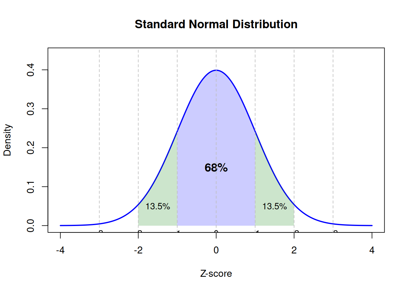
68-95-99.7 rule (empirical rule): Approximately 68% of observations fall within one standard deviation of the mean (μ ± σ), about 95% fall within two standard deviations (μ ± 2σ), and about 99.7% fall within three standard deviations (μ ± 3σ)[1]. This rule provides quick intuition for interpreting z-scores and identifying unusual values.
Code
# Create standard normal curvex <-seq(-4, 4, length =200)y <-dnorm(x, mean =0, sd =1)# Plotplot(x, y, type ="l", lwd =2, col ="blue",xlab ="Z-score", ylab ="Density",main ="Standard Normal Distribution",ylim =c(0, max(y) *1.1))# Shade regions for 68-95-99.7 rule# 68% region (within 1 SD)x1 <-seq(-1, 1, length =100)y1 <-dnorm(x1)polygon(c(-1, x1, 1), c(0, y1, 0), col =rgb(0, 0, 1, 0.2), border =NA)text(0, 0.15, "68%", cex =1.2, font =2)# 95% region (within 2 SD)x2a <-seq(-2, -1, length =50)y2a <-dnorm(x2a)polygon(c(-2, x2a, -1), c(0, y2a, 0), col =rgb(0, 0.5, 0, 0.2), border =NA)x2b <-seq(1, 2, length =50)y2b <-dnorm(x2b)polygon(c(1, x2b, 2), c(0, y2b, 0), col =rgb(0, 0.5, 0, 0.2), border =NA)text(-1.5, 0.05, "13.5%", cex =0.9)text(1.5, 0.05, "13.5%", cex =0.9)# Add vertical linesabline(v =c(-3, -2, -1, 0, 1, 2, 3), lty =2, col ="gray")text(c(-3, -2, -1, 0, 1, 2, 3), -0.02, labels =c("-3", "-2", "-1", "0", "+1", "+2", "+3"), cex =0.9)
Figure 7.1: The standard normal distribution showing the 68-95-99.7 rule
This standard normal distribution (mean = 0, SD = 1) illustrates the empirical rule, which states that approximately 68% of observations fall within one standard deviation of the mean (shaded blue region from z = −1 to z = +1), about 95% fall within two standard deviations (blue + green regions from z = −2 to z = +2), and approximately 99.7% fall within three standard deviations[1]. The curve is perfectly symmetric around zero, and the tails extend infinitely in both directions but contain vanishingly small probabilities. This visual representation helps build intuition for interpreting z-scores: a z-score of +2.0 is unusual (beyond the central 95%), while a z-score of +0.5 is quite typical (well within the central 68%). The shaded regions allow quick probability estimates without consulting tables or software, though for precise calculations, normal distribution tables or statistical software should be used[1,2].
7.3.2 The standard normal distribution
When the mean is 0 and the standard deviation is 1, the result is called the standard normal distribution (also called the z-distribution)[1]. Any normal distribution can be converted to the standard normal by computing z-scores:
\[
z = \frac{x - \mu}{\sigma}
\]
This transformation standardizes the scale, making it possible to use a single reference table (the standard normal table, or z-table; see Appendix: Statistical Tables) to find probabilities for any normal distribution[1,2]. Here’s why this is so powerful: without standardization, you would need a separate probability table for every possible combination of mean and standard deviation. For example, vertical jump height might have μ = 45 cm and σ = 7 cm in one sample, but μ = 52 cm and σ = 9 cm in another sample. Similarly, grip strength might be measured in kilograms with μ = 48 kg and σ = 12 kg. Each of these would require its own unique probability table[1].
The z-score transformation eliminates this problem by expressing every observation in units of standard deviations from the mean, regardless of the original measurement scale[2]. A z-score of +1.5 means “1.5 standard deviations above the mean” whether you’re measuring jump height in centimeters, grip strength in kilograms, or reaction time in milliseconds[3]. This standardization has several important implications for movement science:
Universal comparison: You can compare performance across different tests and variables. An athlete with z = +1.2 on both vertical jump and sprint speed is performing similarly above average on both measures, even though the raw scores (e.g., 55 cm vs. 4.8 seconds) cannot be directly compared[14].
Simplified probability calculations: Once converted to z-scores, all probability calculations use the same standard normal distribution. The probability of exceeding z = +1.96 is always 2.5% (one-tailed), regardless of the original measurement units[1].
Percentile interpretation: Z-scores directly translate to percentiles. A z-score of 0 is always the 50th percentile, z = +1.0 is approximately the 84th percentile, and z = -1.0 is approximately the 16th percentile, making normative comparisons straightforward[2,3].
Cross-study comparison: When researchers report results as standardized effect sizes (e.g., Cohen’s d, which is conceptually similar to a z-score), you can compare findings across studies that used different measurement instruments or populations[13].
In practical terms, this means that once you master the standard normal distribution, you can work with any normally distributed variable simply by converting to z-scores first[1,2].
ImportantWhy the normal distribution matters
The normal distribution is fundamental to statistical inference for three reasons:
Many natural processes produce approximately normal distributions, especially when outcomes result from the sum of many small, independent random effects (Central Limit Theorem, covered in Chapter 8)[1,7].
Mathematical tractability: The normal distribution has convenient mathematical properties that make calculations (means, variances, sums) straightforward[1].
Foundation for inference: Many statistical procedures (t-tests, ANOVA, regression) assume that errors or sampling distributions are approximately normal, even when raw data are not[2,6].
7.4 Using the normal distribution to find probabilities
One of the most practical uses of the normal distribution is converting z-scores to probabilities and percentiles. This connection allows us to answer questions like “What percentage of athletes jump higher than 50 cm?” or “What jump height corresponds to the 90th percentile?” when the variable is approximately normally distributed[1,3].
7.4.1 From z-scores to probabilities
If a variable is approximately normal, we can use the standard normal distribution to find the probability that an observation falls in a particular range[1]. The steps are:
Use a standard normal table (see Appendix: Statistical Tables), calculator, or software to find the cumulative probability.
Interpret the result as a proportion or percentage.
7.4.1.1 Worked example: Finding the probability of an observation
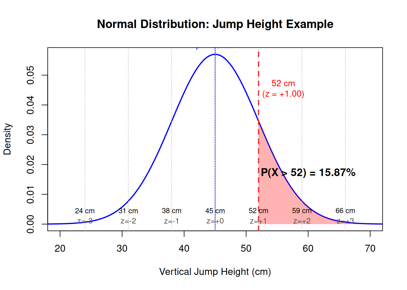
Suppose vertical jump heights are known to be approximately normally distributed in a population of collegiate athletes with mean μ = 45 cm and standard deviation σ = 7 cm. What proportion of athletes in this population jump higher than 52 cm?
Step 1: Compute the z-score
\[
z = \frac{52 - 45}{7} = \frac{7}{7} = 1.00
\]
Step 2: Find the cumulative probability
Using a standard normal table (see Appendix: Statistical Tables or use my interactive z-score calculator), the cumulative probability for z = 1.00 is approximately 0.8413. This means 84.13% of the distribution falls at or below z = 1.00[1].
Step 3: Compute the upper tail probability
Since we want the proportion above 52 cm:
\[
P(X > 52) = 1 - 0.8413 = 0.1587
\]
Interpretation
Approximately 15.87% of athletes in this population jump higher than 52 cm, assuming jump heights are normally distributed with the given mean and standard deviation.
Code
# Parametersmu <-45sigma <-7x_threshold <-52z_threshold <- (x_threshold - mu) / sigma# Create normal curvex <-seq(mu -4*sigma, mu +4*sigma, length =200)y <-dnorm(x, mean = mu, sd = sigma)# Plotplot(x, y, type ="l", lwd =2, col ="blue",xlab ="Vertical Jump Height (cm)", ylab ="Density",main ="Normal Distribution: Jump Height Example",xlim =c(20, 70))# Shade upper tail (above 52 cm)x_upper <-seq(x_threshold, max(x), length =100)y_upper <-dnorm(x_upper, mean = mu, sd = sigma)polygon(c(x_threshold, x_upper, max(x)), c(0, y_upper, 0), col =rgb(1, 0, 0, 0.3), border =NA)# Add vertical line at thresholdabline(v = x_threshold, lty =2, lwd =2, col ="red")text(x_threshold +4, max(y) *0.8, "52 cm\n(z = +1.00)", cex =0.9, col ="red")# Add text for probabilitytext(x_threshold +8, max(y) *0.3, "P(X > 52) = 15.87%", cex =1.1, font =2)# Add mean lineabline(v = mu, lty =1, lwd =1, col ="blue")text(mu, max(y) *1.05, "μ = 45 cm", cex =0.9, col ="blue")# Add z-score markersz_values <-c(-3, -2, -1, 0, 1, 2, 3)x_positions <- mu + z_values * sigmaabline(v = x_positions, lty =3, col ="gray70")text(x_positions, max(y) *0.08, labels =paste0(round(x_positions), " cm"),cex =0.75, col ="black")text(x_positions, max(y) *0.02, labels =paste0("z=", ifelse(z_values >=0, "+", ""), z_values),cex =0.8, col ="gray30")
Figure 7.2: Normal distribution showing the probability of jumping higher than 52 cm (z = 1.00)
This visualization illustrates how the normal distribution connects z-scores to probabilities. The vertical red line marks 52 cm (z = +1.00), and the shaded red region represents the upper tail probability (15.87%) of jumping higher than this value[1]. The mean (μ = 45 cm) is marked with a blue vertical line at the center of the distribution. When jump heights are approximately normally distributed, the area under the curve to the right of 52 cm directly corresponds to the proportion of athletes expected to exceed that height. This graphical approach reinforces the interpretation: values farther from the mean (larger |z|) are less common, and the proportion in the tails decreases as we move outward. Such probability calculations are fundamental to normative assessments, percentile-based classifications, and understanding the rarity of extreme performances in Movement Science contexts[3,11].
7.4.2 From probabilities to raw scores (finding percentiles)
We can also work backward: given a desired probability or percentile rank, find the corresponding z-score and then convert to the raw score scale[1].
7.4.2.1 Worked example: Finding the 90th percentile
Using the same jump height distribution (μ = 45 cm, σ = 7 cm), what jump height corresponds to the 90th percentile?
Step 1: Find the z-score for the 90th percentile
Using a standard normal table (see Appendix: Statistical Tables) or software, the z-score that corresponds to a cumulative probability of 0.90 is approximately z = 1.28[1].
The 90th percentile jump height is approximately 54 cm. This means 90% of athletes jump 54 cm or lower, and 10% jump higher than 54 cm, under the assumption of a normal distribution.
WarningCommon mistake
Treating all Movement Science variables as if they are normally distributed. Many variables (reaction time, sway area, EMG amplitude) are systematically skewed and do not follow a normal distribution[4,5]. Always visualize before assuming normality.
7.5 Skewness: asymmetry in distributions
Skewness quantifies the degree of asymmetry in a distribution[1,15]. A perfectly symmetric distribution (like the normal distribution) has skewness = 0. Positive skewness indicates a right-skewed distribution (long tail to the right), while negative skewness indicates a left-skewed distribution (long tail to the left)[2].
7.5.1 Interpreting skewness values
While there are different formulas for calculating skewness, a common interpretation guideline for sample skewness is[2,16]:
|Skewness| < 0.5: Approximately symmetric (negligible skew)
0.5 ≤ |Skewness| < 1.0: Moderate skew
|Skewness| ≥ 1.0: High skew (substantial asymmetry)
In Movement Science, right skew is common: reaction times are bounded below by physiological limits but can be very long if attention lapses; sway area cannot be negative but can be very large during instability; EMG amplitude is strictly positive and often shows occasional large bursts[5,17].
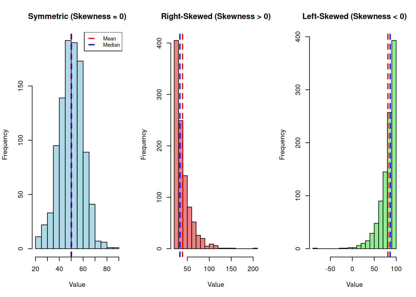
Figure 7.3: Examples of symmetric, right-skewed, and left-skewed distributions
These histograms illustrate different patterns of skewness commonly encountered in Movement Science data[2,18]. The symmetric distribution (left panel) shows mean and median nearly overlapping, consistent with approximate normality. The right-skewed distribution (center panel) shows the mean pulled toward the long right tail, exceeding the median—a pattern typical of reaction times, sway area, and EMG amplitude where values cannot be negative but occasional large values occur[5]. The left-skewed distribution (right panel) shows the mean pulled toward the long left tail, below the median—less common in movement data but can occur with ceiling-bounded measures like function scores where many participants cluster near the maximum[18]. Recognizing skewness visually helps determine whether mean-based summaries are appropriate or whether medians, transformations, or nonparametric methods are preferable[6,8].
7.5.3 Worked example: Computing skewness
Most statistical software computes skewness automatically. For a small dataset, skewness can be approximated by observing the relationship between mean and median:
If mean ≈ median: symmetric (skewness ≈ 0)
If mean > median: right-skewed (positive skewness)
If mean < median: left-skewed (negative skewness)
For a dataset of reaction times (in milliseconds):
Since mean > median (250.56 > 245), this suggests right skew. The value 320 ms is an outlier that pulls the mean upward, a common pattern in reaction time data[2,5].
7.5.4 Testing the significance of skewness: z-skew
While rules of thumb for interpreting skewness values are helpful, a more precise approach is to compute the z-score for skewness (often called z-skew), which tests whether the observed skewness is statistically different from zero[2,19].
where \(SE_{\text{skew}}\) is the standard error of skewness, typically provided by statistical software alongside the skewness value.
Interpretation:
If \(|z_{\text{skew}}| < 1.96\): Skewness is not significant at α = 0.05 (distribution is approximately symmetric)
If \(|z_{\text{skew}}| \geq 1.96\): Skewness is significant at α = 0.05 (distribution shows statistically significant asymmetry)
If \(|z_{\text{skew}}| \geq 2.58\): Skewness is highly significant at α = 0.01
Example:
Suppose SPSS reports:
Skewness = 0.45
Std. Error = 0.31
\[
z_{\text{skew}} = \frac{0.45}{0.31} = 1.45
\]
Since \(|1.45| < 1.96\), the skewness is not statistically significant at α = 0.05. Although the distribution shows slight positive skew (0.45), this could easily occur by chance with normal data in samples of this size[2].
Contrast with a clearly skewed example:
Skewness = 1.85
Std. Error = 0.31
\[
z_{\text{skew}} = \frac{1.85}{0.31} = 5.97
\]
Since \(|5.97| \geq 2.58\), the skewness is highly significant (p < .01), providing strong evidence of right-skewed distribution requiring attention (e.g., transformation or nonparametric methods)[6,9].
ImportantSample size matters
With very large samples (n > 200), even trivial skewness (e.g., 0.15) can become statistically significant due to increased statistical power[7]. Conversely, with small samples (n < 30), substantial skewness may fail to reach significance due to large standard errors. Always interpret z-skew in combination with the magnitude of skewness and visual assessment[2,8].
7.6 Kurtosis: tail weight and peakedness
Kurtosis quantifies the “tailedness” or extremity of a distribution relative to the normal distribution[1,15,20]. Historically, kurtosis was described as “peakedness,” but modern interpretation emphasizes tail weight: distributions with high kurtosis have heavy tails (more extreme values) and a sharper peak, while distributions with low kurtosis have light tails (fewer extreme values) and a flatter peak[20].
Leptokurtic (kurtosis > 0): Heavy tails with more extreme values than a normal distribution; sharper peak[20].
Platykurtic (kurtosis < 0): Light tails with fewer extreme values than a normal distribution; flatter peak[20].
Note: Some software reports “excess kurtosis” (kurtosis − 3), where a normal distribution has excess kurtosis = 0. Other software reports raw kurtosis, where a normal distribution has kurtosis = 3. Always verify which version your software uses[2,15].
7.6.2 Why kurtosis matters in Movement Science
Leptokurtic distributions (heavy tails) can produce more extreme outliers than expected under normality, which matters for identifying unusual performances and for the behavior of mean-based statistics[20]. For example, if strength measurements occasionally include a few extremely high or low values due to motivational factors or measurement artifacts, the distribution may appear leptokurtic, indicating that outliers are more common than a normal model predicts[8].
Platykurtic distributions (light tails) indicate fewer extremes, which can occur when outcomes are constrained or when subgroups with different means are combined, flattening the overall distribution[2].
7.6.3 Testing the significance of kurtosis: z-kurtosis
Similar to z-skew, we can compute the z-score for kurtosis (often called z-kurtosis or z-kurt) to test whether the observed kurtosis departs significantly from normal tail behavior[2,19].
Since \(|-0.36| < 1.96\), the kurtosis is not statistically significant. The distribution shows slightly lighter tails than a perfect normal distribution, but this is well within sampling variability[2].
Since \(|5.61| \geq 2.58\), the kurtosis is highly significant (p < .01), indicating that the distribution has substantially heavier tails than a normal distribution, with more extreme values than expected[8,20]. This suggests increased caution when interpreting outliers and when relying on mean-based statistics.
NoteReal example: reaction time distributions
Reaction times are typically right-skewed (positive skewness) and leptokurtic (heavy right tail). The right skew reflects that responses cannot be faster than physiological limits (~100–150 ms) but can be much slower if attention lapses. The heavy tail reflects occasional very slow responses, making the distribution more “long-tailed” than a normal curve would predict[5]. For this reason, median reaction time is often more representative than mean, and robust methods are preferred when modeling reaction time data[3,8].
Quantitatively, if skewness = 1.85 (SE = 0.31), then z-skew = 5.97, and if kurtosis = 3.42 (SE = 0.61), then z-kurt = 5.61—both highly significant, providing strong statistical evidence that reaction times violate normality assumptions and require alternative methods[6,9].
7.6.4 Interpreting z-skew and z-kurtosis together
When assessing distributional shape, consider both z-skew and z-kurtosis together[2]:
z-skew
z-kurt
Interpretation
Action
< 1.96
< 1.96
Approximately normal
Parametric methods appropriate
≥ 1.96
< 1.96
Significant asymmetry, normal tails
Consider transformation or nonparametric tests
< 1.96
≥ 1.96
Symmetric but abnormal tails
Use robust methods or check for outliers
≥ 1.96
≥ 1.96
Both skewed and heavy/light tails
Transformation or nonparametric methods recommended
This combined approach provides a more nuanced assessment than relying on a single measure alone[19,21].
7.7 Assessing normality visually
Before running formal normality tests, always visualize the distribution. Visual assessment is often more informative than a single p-value because it shows the pattern and magnitude of departure from normality[2,10,22].
7.7.1 Histograms with normal overlay
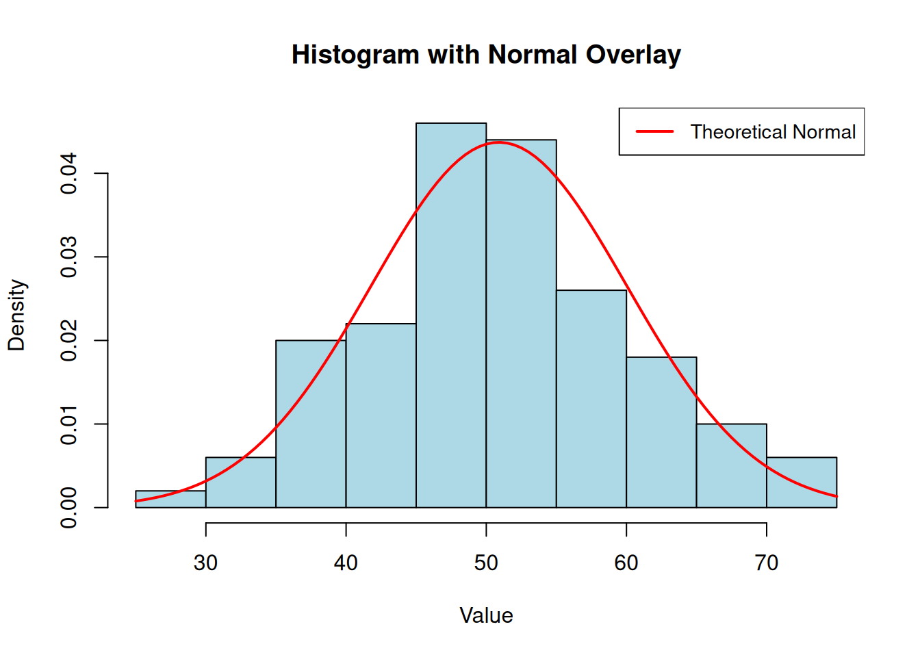
A histogram with a superimposed normal curve allows quick visual comparison between the observed data and a theoretical normal distribution with the same mean and standard deviation[2].
Code
# Generate approximately normal dataset.seed(123)data <-rnorm(100, mean =50, sd =10)# Histogramhist(data, breaks =15, col ="lightblue", border ="black", probability =TRUE,main ="Histogram with Normal Overlay", xlab ="Value", ylab ="Density")# Overlay normal curvecurve(dnorm(x, mean =mean(data), sd =sd(data)), col ="red", lwd =2, add =TRUE)legend("topright", legend ="Theoretical Normal", col ="red", lwd =2, cex =0.9)
Figure 7.4: Histogram with normal curve overlay for approximately normal data
This histogram shows data that closely follow a normal distribution. The red curve represents a theoretical normal distribution with the same mean and standard deviation as the observed data. When the histogram bars align well with the curve, approximate normality is supported[2]. Deviations appear as gaps (fewer observations than expected) or excess bars (more observations than expected) relative to the curve. For Movement Science applications, perfect alignment is never achieved, but close correspondence suggests that mean-based summaries and normal-theory inference are reasonable[1,7].
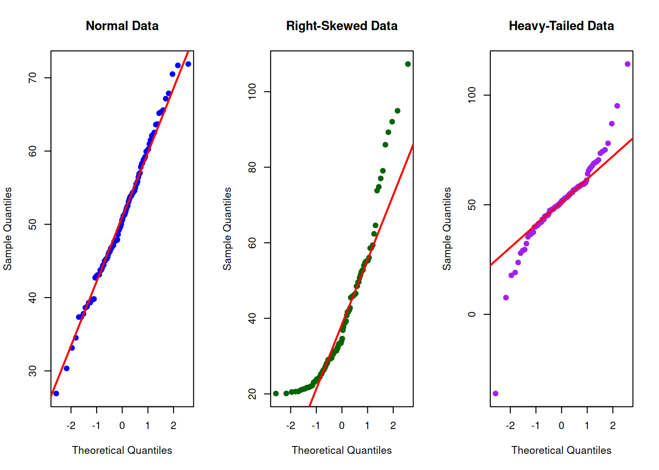
7.7.2 Q-Q plots (Quantile-Quantile plots)
A Q-Q plot (quantile-quantile plot) is one of the most effective tools for assessing normality[1,2,8]. It plots the observed data quantiles against the quantiles expected from a normal distribution. If the data are approximately normal, the points fall close to a straight diagonal line[2].
How to interpret Q-Q plots:
Points close to the line: Data are approximately normal.
Points curve upward at the ends: Heavy tails (leptokurtic).
Points curve downward at the ends: Light tails (platykurtic).
S-shaped pattern: Skewed distribution.
Few extreme points off the line: Possible outliers, but overall distribution may still be reasonable[2,8].
Code
par(mfrow =c(1, 3))# Normal dataset.seed(123)normal_data <-rnorm(100, mean =50, sd =10)qqnorm(normal_data, main ="Normal Data", pch =19, col ="blue")qqline(normal_data, col ="red", lwd =2)# Right-skewed dataskewed_data <-rexp(100, rate =0.05) +20qqnorm(skewed_data, main ="Right-Skewed Data", pch =19, col ="darkgreen")qqline(skewed_data, col ="red", lwd =2)# Heavy-tailed dataheavy_data <-rt(100, df =3) *10+50qqnorm(heavy_data, main ="Heavy-Tailed Data", pch =19, col ="purple")qqline(heavy_data, col ="red", lwd =2)par(mfrow =c(1, 1))
Figure 7.5: Q-Q plots for normal, right-skewed, and heavy-tailed distributions
These Q-Q plots illustrate different patterns of departure from normality[2,8]. The left panel shows approximately normal data: points cluster tightly around the diagonal reference line, indicating observed quantiles match expected normal quantiles. The center panel shows right-skewed data: points curve upward at the right end, reflecting the long right tail characteristic of many Movement Science variables like reaction time and sway area[5]. The right panel shows heavy-tailed (leptokurtic) data: points deviate from the line at both extremes, indicating more extreme values than expected under normality[20]. Q-Q plots are more sensitive than histograms for detecting departures from normality and are strongly recommended before assuming normality for inference[1,19]. In practice, minor deviations are common and often inconsequential, especially with larger samples, but systematic patterns (strong curvature, S-shapes) suggest that normality assumptions may be problematic[6,7].
TipPractical advice: trust your eyes
A Q-Q plot showing slight waviness or a few points off the line does not necessarily mean you must abandon normal-theory methods, especially with moderate to large samples (n > 30). Look for substantial, systematic departures (strong curves, S-shapes) rather than treating minor wiggles as fatal flaws[2,7,22].
7.8 Formal tests of normality
Formal normality tests provide p-values that quantify evidence against the normality assumption[19,23]. Common tests include:
Shapiro-Wilk test: Generally considered the most powerful test for normality, especially in small to moderate samples[19,21,23].
Kolmogorov-Smirnov test: Tests whether the observed distribution matches a specified distribution (e.g., normal). Less powerful than Shapiro-Wilk[19,21].
Anderson-Darling test: Similar to Kolmogorov-Smirnov but gives more weight to tails[21].
7.8.1 How normality tests work
Normality tests evaluate the null hypothesis that the data come from a normal distribution[19,23]:
\(H_0\): The data are normally distributed.
\(H_A\): The data are not normally distributed.
A small p-value (typically p < 0.05) suggests evidence against normality; you reject the null hypothesis and conclude the data are not normally distributed[19,23]. A large p-value suggests insufficient evidence to reject normality, though it does not prove normality[2,19].
7.8.2 Limitations of normality tests
Formal normality tests have important limitations that can lead to misinterpretation if used mechanically[2,7,19]:
Sample size sensitivity: With small samples (n < 30), normality tests have low power and may fail to detect clear departures. With large samples (n > 100), tests become very sensitive and may reject normality for trivial departures that have no practical impact on inference[2,7].
Binary decision trap: A p-value near 0.05 does not indicate “borderline normality.” Distributions can be “normal enough” even when p < 0.05, or “problematic” even when p > 0.05, depending on the context and planned analysis[6,19].
Visual assessment is often better: Experienced analysts prioritize Q-Q plots and histograms over p-values because visual methods reveal the pattern and magnitude of departure, not just a binary “reject/fail to reject” decision[2,10,22].
WarningCommon mistake
Relying solely on normality test p-values to decide whether to use parametric methods. With large samples, trivial departures can produce p < 0.05, while with small samples, substantial departures can produce p > 0.05. Always combine formal tests with visual assessment and consider the robustness of your planned analysis[2,6,7].
7.8.3 Worked example: Interpreting a Shapiro-Wilk test
Suppose you run a Shapiro-Wilk test on a sample of 50 sprint times and obtain:
W = 0.964, p = 0.132
Interpretation:
The p-value (0.132) is greater than the conventional threshold of 0.05, so we fail to reject the null hypothesis of normality. This suggests insufficient evidence to conclude that sprint times are non-normal. However, this does not prove normality. You should also examine a Q-Q plot and histogram to confirm that the distribution appears approximately normal and that any departures are minor[2,19,23].
Conversely, if the Shapiro-Wilk test yields p = 0.003, you would reject normality. In this case, visual inspection should reveal the pattern of departure (skew, heavy tails, outliers). If the departure is severe, consider using robust methods, transformations, or nonparametric alternatives[6,8].
7.9 When movement data are not normal
Many Movement Science variables systematically deviate from normality, and recognizing these patterns is essential for choosing appropriate summaries and analyses[4–6].
7.9.1 Common patterns of non-normality in Movement Science
Right-skewed variables (positive skew, long right tail):
Reaction times: Bounded below by physiology (~100 ms) but can be very long[5]
Sway area, sway path length: Cannot be negative, occasional large values during instability[17]
EMG amplitude: Strictly positive, bursts can be much larger than baseline[5]
Fatigue indices: Often show ceiling effects (maximum fatigue) with occasional high values
Ceiling or floor effects (truncation):
Function scores (e.g., 0–100 scales) where many participants cluster at the upper bound[2]
Pain scales (e.g., 0–10) where many report low pain (floor effect) or maximum pain (ceiling effect)
Strength tests where measurement limits are reached
Bimodal or multimodal distributions:
Mixed samples with distinct subgroups (e.g., combining trained and untrained participants)[10]
Different movement strategies producing separate clusters[17]
Measurement artifacts creating distinct peaks (e.g., digit preference, rounding)
Heavy-tailed distributions (leptokurtic):
Strength tests with occasional extreme efforts
Balance tests where most performances are stable but a few show dramatic instability
Data including measurement errors or motivational outliers[8,20]
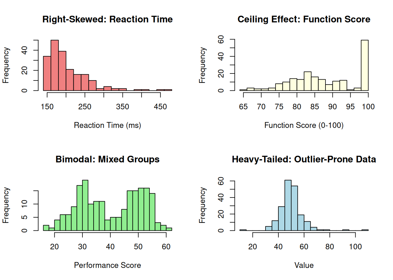
Figure 7.6: Common patterns of non-normality in Movement Science data
These histograms illustrate common non-normal patterns in Movement Science data[4,6]. The right-skewed reaction time distribution (top-left) shows the characteristic long right tail due to physiological lower bounds and occasional lapses in attention[5]. The ceiling effect (top-right) shows many participants clustered at the maximum function score, creating a pile-up that violates normality and can obscure meaningful differences[2]. The bimodal distribution (bottom-left) reflects two distinct subgroups (e.g., trained vs. untrained), suggesting that analyzing them separately would be more informative than combining them[10]. The heavy-tailed distribution (bottom-right) shows more extreme values than expected under normality, indicating greater susceptibility to outliers—common in strength and fatigue measures where motivation or measurement artifacts can produce unusual values[8,20]. Recognizing these patterns helps determine whether transformations, robust methods, or nonparametric approaches are preferable to standard parametric analyses[6,7].
7.9.2 What to do when data are not normal
When visual and formal assessments reveal substantial departures from normality, several principled options exist[2,6,8]:
Use robust or nonparametric methods:
Median and IQR instead of mean and SD for summaries[8]
Mann-Whitney U or Kruskal-Wallis tests instead of t-tests or ANOVA (see Chapter 19)[2]
Bootstrapping or permutation tests for inference[8]
Transform the variable:
Log transformation for right-skewed, ratio-scale variables (reaction time, sway area, EMG amplitude)[5,24]
Square root or Box-Cox transformations for count data
Report results on the transformed scale or back-transform carefully[24]
Accept the departure and proceed with caution:
Many procedures (t-tests, ANOVA) are reasonably robust to moderate departures, especially with larger samples (n > 30) and balanced designs[6,7]
Use Welch’s t-test instead of Student’s t-test when variances differ[9]
Focus on effect sizes and confidence intervals rather than p-values[22,25]
Separate subgroups:
If bimodality reflects distinct groups, analyze them separately rather than combining[10]
Acknowledge and report:
Describe the distributional shape, note the departure from normality, and justify your analytic approach[2]
NoteReal example: reaction time analysis
A researcher collects reaction times and finds strong right skew (skewness = 1.8) and a Shapiro-Wilk p-value of 0.002. The Q-Q plot shows clear upward curvature at the right end. Options:
Log transform: \(\log(\text{RT})\) often normalizes reaction time data, allowing parametric methods on the transformed scale[5,24].
Use median: Report median reaction time with IQR, avoid mean-based comparisons[8].
Nonparametric test: Use Mann-Whitney U or Kruskal-Wallis for group comparisons (Chapter 19)[2].
The researcher chooses log transformation, confirms approximate normality on the log scale, and proceeds with t-tests on log(RT), then back-transforms results to communicate findings as geometric means and ratios[5,24].
7.10 Integrating multiple lines of evidence
A common dilemma arises when visual assessments (histograms, Q-Q plots) and formal statistical tests (Shapiro-Wilk, z-skew, z-kurtosis) yield conflicting conclusions about normality. For example, a Q-Q plot may show points closely following the reference line while the Shapiro-Wilk test returns p < 0.05, or conversely, visual inspection reveals clear departure while formal tests fail to reject normality. How should researchers navigate these conflicts?[2,7,19]
7.10.1 Why conflicts occur: the sample size paradox
The primary reason for conflicting results lies in how formal tests respond to sample size[19,21]:
Large samples (n > 100): Formal tests become extremely sensitive, detecting trivially small departures from perfect normality that have no practical impact on parametric procedures. A histogram and Q-Q plot may show near-perfect normality, yet p < 0.001 because the test has sufficient power to detect deviations that are statistically significant but practically irrelevant[2,7].
Small samples (n < 30): Formal tests have low statistical power, often failing to detect meaningful departures. Visual methods may reveal obvious skew or outliers, yet p > 0.05 simply because the sample is too small for the test to achieve significance[1,21].
This creates a paradox: formal tests are most reliable when you need them least (moderate sample sizes) and least reliable when you need them most (very small or very large samples)[2,19].
7.10.2 A principled decision framework
Rather than relying on any single method, integrate all available evidence using this hierarchical approach[2,7,8]:
7.10.2.1Step 1: Prioritize visual assessment
Visual methods (histograms, Q-Q plots) provide the nature and magnitude of departure, not just a binary “normal or not” verdict. They reveal whether data are:
Mildly skewed vs. severely skewed
Symmetric with one outlier vs. systematically heavy-tailed
Approximately normal with minor waviness vs. clearly bimodal[2,10]
This information guides action (e.g., log transformation for right-skew, robust methods for outliers, separate analyses for bimodality) in ways that formal tests cannot[6,8].
7.10.2.2Step 2: Consider sample size when interpreting formal tests
n < 30: Weight visual assessment heavily. Formal tests may lack power to detect real departures. If visuals show clear non-normality (e.g., obvious skew, multiple outliers), act on it even if p > 0.05[2,21].
30 ≤ n < 100: Formal tests are most informative in this range. Balance formal and visual evidence, using z-skew and z-kurtosis to quantify magnitude[16,19].
n ≥ 100: Weight visual assessment heavily again. Formal tests may detect trivial departures. If visuals show approximate normality but p < 0.05, consider proceeding with parametric methods (especially robust variants like Welch’s t-test) since large samples invoke the Central Limit Theorem[7,9].
7.10.2.3Step 3: Evaluate practical vs. statistical significance
A statistically significant departure (p < 0.05) is not necessarily a practically important one. Ask:
Is the skewness moderate (|skew| < 1) or extreme (|skew| > 2)?[16]
Do diagnostic plots show systematic departure or minor waviness?[2]
Will the planned analysis (e.g., Welch’s t-test, bootstrapping) be robust to the observed departure?[8,9]
7.10.2.4Step 4: Apply the convergence rule
All methods agree (visual + formal): High confidence in conclusion. Proceed accordingly.
Visual shows normality, formal tests reject: Likely due to large sample size detecting trivial deviations. Trust visual assessment; proceed with parametric methods (especially if n > 100)[2,7].
Visual shows departure, formal tests do not reject: Likely due to low power in small samples. Trust visual assessment; use transformation, robust methods, or nonparametric approaches[8,21].
Borderline/ambiguous: Use robust methods (e.g., Welch’s t-test, bootstrapping) that perform well under both normality and moderate departures, or report parallel analyses with parametric and nonparametric methods[8,9].
7.10.3 Decision table for conflicting evidence
Visual Assessment
Formal Test Result
Sample Size
Recommended Action
Approximately normal
p < 0.05
n < 30
Use parametric methods; test likely underpowered
Approximately normal
p < 0.05
n ≥ 100
Use parametric methods; trivial departure detected
Clear departure
p > 0.05
n < 30
Transform or use robust/nonparametric methods
Clear departure
p > 0.05
n ≥ 100
Investigate data quality; consider transformation
Mild departure
p < 0.05
Any
Use robust methods (Welch’s t, bootstrap); report effect sizes
Severe departure
p < 0.05
Any
Transform, use nonparametric methods, or separate groups
ImportantThe primacy of visual assessment
Modern statistical practice emphasizes that visual assessment should be the primary tool for evaluating normality, with formal tests serving as supplementary evidence[2,7,8]. This recommendation reflects:
Visual methods reveal what is wrong, formal tests only whether something is wrong.
The practical impact of departures cannot be judged from p-values alone.
Sample size strongly influences formal test results independent of the departure’s magnitude.
Expert judgment about distributional shape is more informative than mechanical application of significance thresholds[10,19].
However, this does not mean formal tests should be ignored. They provide useful quantification (z-skew, z-kurtosis) and can detect subtle departures that might be missed visually. The key is integration, not exclusion[2,21].
WarningCommon mistake: over-reliance on p-values
A p-value from a normality test should never be the sole basis for decisions about analysis strategy. A researcher who uses a Shapiro-Wilk p < 0.05 to reject mean-based summaries for data with n = 200, mild skewness (skew = 0.4), and a histogram showing near-perfect bell shape is likely discarding valuable information unnecessarily. Conversely, accepting normality based solely on p > 0.05 when n = 15 and the Q-Q plot shows clear curvature risks violating assumptions when they truly matter[2,19,21].
7.11 When normality assumptions matter most
Understanding when departures from normality are consequential helps prioritize where to invest effort in assessment and remediation[6,7,9]:
7.11.1 High priority: check normality carefully
Small samples (n < 30): Parametric methods rely more heavily on distributional assumptions when samples are small[1,2].
Hypothesis tests with extreme p-values near cutoffs: If your inference hinges on p = 0.048 vs. p = 0.052, normality violations could tip the decision[19].
Variables known to be non-normal: Reaction time, sway area, EMG amplitude should be scrutinized rather than assumed normal[3,5].
7.11.2 Lower priority: normality less critical
Large samples (n > 100): The Central Limit Theorem ensures that sampling distributions of means are approximately normal even when raw data are not, making parametric tests robust[1,7].
Moderate departures with robust methods: If using Welch’s t-test, rank-based methods, or bootstrap inference, exact normality is less critical[8,9].
Descriptive summaries: When the goal is description (not inference), median and IQR can be reported regardless of normality[2].
ImportantKey principle: context over rules
There is no universal rule for “how normal is normal enough.” The answer depends on:
Sample size: Larger samples tolerate more departure.
Purpose: Inference requires stronger assumptions than description.
Magnitude of departure: Slight skew ≠ extreme bimodality.
Robustness of method: Some procedures (Welch’s t-test, bootstrapping) are inherently more forgiving[7–9].
7.12 Worked example using the Core Dataset
This example demonstrates a complete normality assessment workflow for a Movement Science variable.
7.12.1 Scenario: Assessing normality of sprint times
A researcher collects 20-meter sprint times from 40 participants. Before conducting a t-test to compare two training groups, they assess normality.
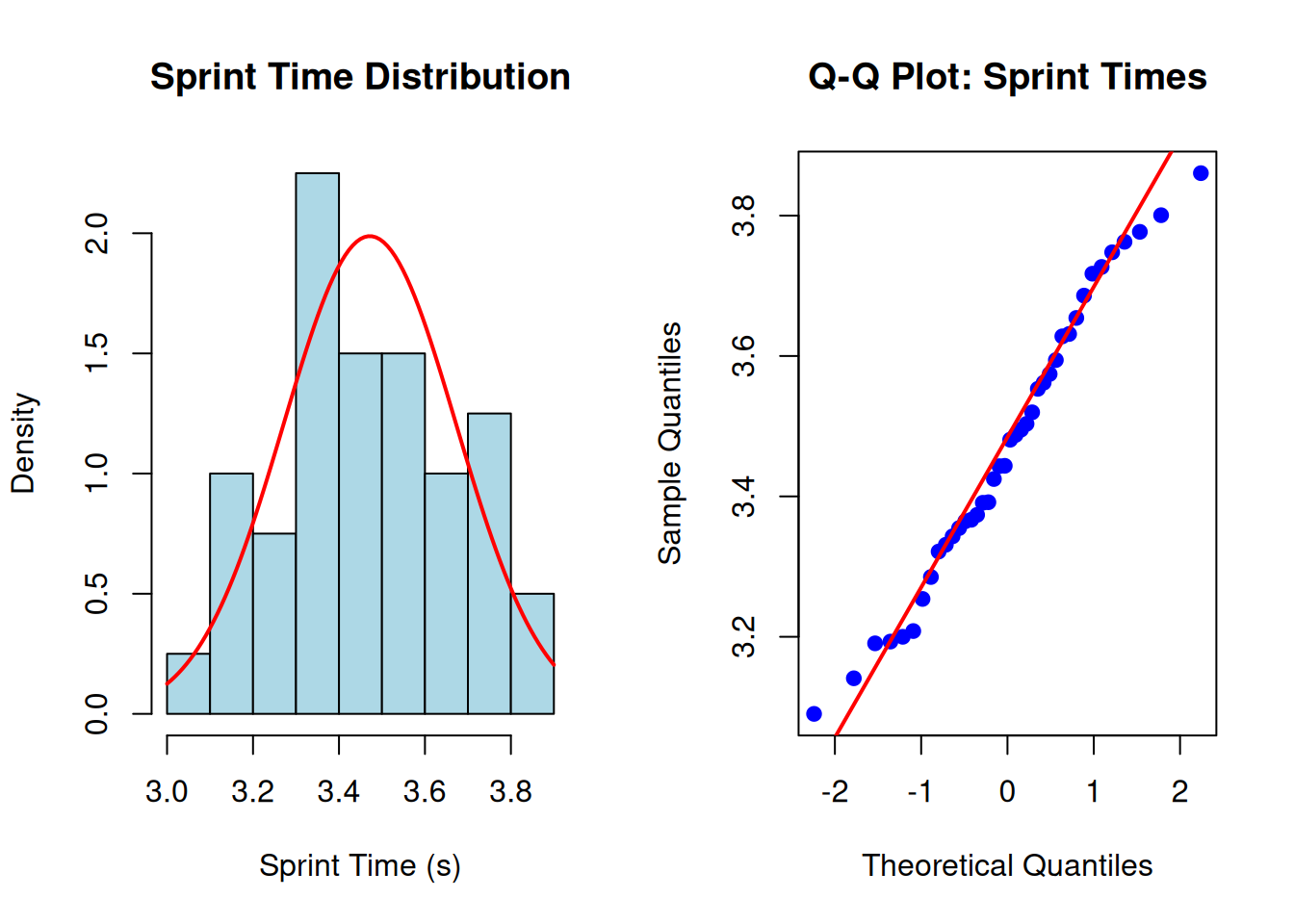
Step 1: Visualize with histogram and Q-Q plot
Code
# Simulate sprint time data (approximately normal)set.seed(456)sprint <-rnorm(40, mean =3.45, sd =0.18)par(mfrow =c(1, 2))# Histogram with normal overlayhist(sprint, breaks =10, col ="lightblue", border ="black", probability =TRUE,main ="Sprint Time Distribution", xlab ="Sprint Time (s)", ylab ="Density")curve(dnorm(x, mean =mean(sprint), sd =sd(sprint)), col ="red", lwd =2, add =TRUE)# Q-Q plotqqnorm(sprint, main ="Q-Q Plot: Sprint Times", pch =19, col ="blue")qqline(sprint, col ="red", lwd =2)par(mfrow =c(1, 1))
Figure 7.7: Normality assessment for sprint times: histogram and Q-Q plot
Interpretation: The histogram shows reasonable symmetry with no extreme outliers. The Q-Q plot shows points close to the diagonal line with minor waviness at the ends—consistent with approximate normality[1,2].
Step 2: Compute skewness and kurtosis
(Using software)
Skewness = 0.15 (negligible)
Kurtosis = −0.22 (close to normal)
Interpretation: Both values are close to zero, supporting approximate normality[15,16].
Step 3: Run Shapiro-Wilk test
W = 0.975, p = 0.524
Interpretation: p > 0.05 indicates insufficient evidence to reject normality. Combined with visual assessment, the data appear approximately normal[19,23].
Step 4: Decision
Proceed with parametric t-test. The distribution is approximately normal, and the sample size (n = 40) provides additional robustness[1,7].
7.13 Chapter summary
The normal distribution is a symmetric, bell-shaped probability distribution characterized by its mean and standard deviation, and it plays a foundational role in statistical inference because many procedures assume normality of errors or sampling distributions[1,2]. The empirical rule (68-95-99.7) provides intuition for interpreting z-scores, and the standard normal distribution allows conversion between z-scores, probabilities, and percentiles[1]. Skewness quantifies asymmetry, with right skew (positive values) common in Movement Science variables like reaction time, sway area, and EMG amplitude, while kurtosis quantifies tail weight, with heavy-tailed distributions producing more extreme outliers than expected under normality[5,15,20]. Assessing normality requires both visual methods (histograms with normal overlays, Q-Q plots) and, when appropriate, formal tests like the Shapiro-Wilk test, though visual assessment is often more informative than p-values alone because it reveals patterns and magnitudes of departure[2,10,19,22]. Many Movement Science variables systematically deviate from normality due to biological constraints, measurement properties, or task structure, and recognizing these patterns allows informed decisions about whether to transform data, use robust or nonparametric methods, or acknowledge departures while proceeding cautiously with parametric approaches[4,6–8]. The key principle is that “normality” is a continuum, not a binary state: the practical question is whether departures are consequential for the planned analysis and interpretation, with the answer depending on sample size, purpose, magnitude of departure, and robustness of methods[2,7,9].
7.14 Key terms
normal distribution; bell curve; Gaussian distribution; standard normal distribution; z-distribution; empirical rule; 68-95-99.7 rule; probability density function; skewness; kurtosis; mesokurtic; leptokurtic; platykurtic; Q-Q plot; normality test; Shapiro-Wilk test; Kolmogorov-Smirnov test; right-skewed; left-skewed; ceiling effect; floor effect; bimodal distribution; heavy tails; robust methods
7.15 Practice: quick checks
The values 40 and 60 are both exactly one standard deviation from the mean (40 = 50 − 10, and 60 = 50 + 10). According to the empirical rule (68-95-99.7 rule), approximately 68% of observations fall within one standard deviation of the mean in a normal distribution[1]. Therefore, about 68% of observations fall between 40 and 60. This illustrates why the empirical rule is useful for quick probability estimates without consulting tables or software, though for more precise calculations (e.g., for non-integer z-scores), normal distribution tables or software should be used.
The p-value of 0.03 is less than the conventional threshold of 0.05, so you would reject the null hypothesis of normality and conclude that there is statistically significant evidence that the data are not normally distributed[19,23]. However, this conclusion alone is insufficient for deciding how to proceed. With a large sample (n = 200), normality tests become very sensitive and can detect trivial departures that have no practical impact on parametric inference[2,7]. You should examine Q-Q plots and histograms to assess the magnitude and pattern of departure. If visual inspection shows only minor deviations (slight skew, a few outliers), parametric methods may still be robust, especially with the large sample size[6]. If visual assessment reveals substantial departures (strong skew, heavy tails, bimodality), consider robust or nonparametric alternatives[8]. The p-value tells you that departure from normality is detectable, not whether it is consequential.
A Q-Q plot (quantile-quantile plot) compares the observed data quantiles to the quantiles expected from a theoretical normal distribution[1,2]. If the data are approximately normal, the points fall close to a straight diagonal reference line. Systematic departures reveal patterns: points curving upward at the right end indicate right skew (common in reaction time, sway area), points curving upward at both ends indicate heavy tails (leptokurtic distribution with more extreme values than expected), S-shaped patterns indicate skewness, and a few isolated points off the line suggest outliers but do not necessarily invalidate normality[2,8]. Q-Q plots are more informative than histograms for detecting subtle departures and are strongly recommended as part of normality assessment[19,22]. Minor waviness is common and usually not problematic, but substantial, systematic curvature suggests that normality assumptions may be questionable.
Reaction times are right-skewed because they are bounded below by physiological limits (approximately 100–150 ms for simple reactions) but have no upper bound—occasional lapses in attention, distractions, or hesitations can produce very slow responses, creating a long right tail[3,5]. The mean reaction time is therefore pulled upward by these slow responses and often exceeds the median, making the median a more representative measure of “typical” reaction time[2,8]. For analysis, this skewness suggests several options: (1) log transformation, which often normalizes reaction time distributions and allows parametric methods on the log scale[5,24]; (2) reporting median and IQR rather than mean and SD for descriptive summaries; (3) using nonparametric tests (Mann-Whitney U, Kruskal-Wallis) for group comparisons to avoid assumptions about normality[2]. Ignoring the skewness and proceeding with untransformed means can result in misleading summaries and inflated sensitivity to outliers.
Parametric methods (t-tests, ANOVA, regression) are often robust to moderate departures from normality, especially under certain conditions[6,7,9]. First, larger samples (typically n > 30 per group) invoke the Central Limit Theorem, which ensures that sampling distributions of means are approximately normal even when raw data are not, making inference more robust[1,7]. Second, if departures are minor (slight skew, skewness < 1.0, Q-Q plot shows only small deviations), the impact on Type I error rates and power is often negligible[6]. Third, some parametric methods are inherently robust to violations: Welch’s t-test tolerates unequal variances and mild non-normality better than Student’s t-test[9], and ANOVA is reasonably robust with balanced designs and moderate departures[6]. Fourth, if you focus on effect sizes and confidence intervals rather than strict p-value cutoffs, minor violations are less consequential[22,25]. However, substantial departures (strong skew, heavy tails, bimodality, small samples) warrant robust or nonparametric alternatives to ensure valid inferences[2,8]. The key is to assess the context—sample size, magnitude of departure, purpose of analysis—rather than applying rigid rules.
Skewness quantifies asymmetry: it measures whether a distribution has a longer tail on the left (negative skew) or right (positive skew), with zero indicating perfect symmetry[2,15]. Kurtosis quantifies tail weight and extremity: it measures whether a distribution has heavier tails (more extreme values, leptokurtic, positive kurtosis) or lighter tails (fewer extreme values, platykurtic, negative kurtosis) compared to a normal distribution, which has kurtosis = 0 (excess kurtosis)[15,20]. Skewness affects the relationship between mean and median (mean > median for right skew), while kurtosis affects the frequency of outliers and the sharpness of the peak. Both are important diagnostics, but skewness is often more visually obvious and has clearer implications for choosing summaries (median vs. mean), while kurtosis is more subtle and primarily affects the behavior of outlier detection and the robustness of mean-based statistics[2,20]. In Movement Science, right skew is very common (reaction time, sway area, EMG amplitude), while high kurtosis (heavy tails) can signal measurement issues or motivational extremes that produce more outliers than expected under normality[5,8].
NoteRead further
For foundational coverage of the normal distribution and its role in inference, see[1] and[2]. For evidence that many real-world datasets depart from normality, see[4]. For normality testing guidance, see[23],[21], and[19]. For practical advice on when departures matter, see[7],[6], and[9]. For Movement Science-specific applications and non-normal data patterns, see[3],[5], and[8].
TipNext chapter
The next chapter introduces probability and sampling error, building on the normal distribution to explain sampling distributions, the Central Limit Theorem, and how we estimate population parameters from samples.
1. Moore, D. S., McCabe, G. P., & Craig, B. A. (2021). Introduction to the practice of statistics (10th ed.). W. H. Freeman; Company.
2. Field, A. (2018). Discovering statistics using IBM SPSS statistics (5th ed.). SAGE Publications.
3. Vincent, W. J. (1999). Statistics in kinesiology.
6. Blanca, M. J., Alarcón, R., Arnau, J., Bono, R., & Bendayan, R. (2013). Non-normal data: Is ANOVA still a valid option? Psicothema, 25(4), 552–557. https://doi.org/10.7334/psicothema2013.552
7. Lumley, T., Diehr, P., Emerson, S., & Chen, L. (2002). The importance of the normality assumption in large public health data sets. Annual Review of Public Health, 23, 151–169. https://doi.org/10.1146/annurev.publhealth.23.100901.140546
8. Wilcox, R. R. (2017). Introduction to robust estimation and hypothesis testing (4th ed.). Academic Press.
9. Delacre, M., Lakens, D., & Leys, C. (2017). Why psychologists should by default use welch’s t-test instead of student’s t-test. International Review of Social Psychology, 30(1), 92–101. https://doi.org/10.5334/irsp.82
10. Tukey, J. W. (1977). Exploratory data analysis. Addison-Wesley.
12. Atkinson, G., & Nevill, A. M. (1998). Statistical methods for assessing measurement error (reliability) in variables relevant to sports medicine. Sports Medicine, 26(4), 217–238. https://doi.org/10.2165/00007256-199826040-00002
13. Cumming, G. (2012). Understanding the new statistics: Effect sizes, confidence intervals, and meta-analysis. Routledge.
14. Batterham, A. M., & Hopkins, W. G. (2006). Making meaningful inferences about magnitudes. International Journal of Sports Physiology and Performance, 1(1), 50–57. https://doi.org/10.1123/ijspp.1.1.50
15. Joanes, D. N., & Gill, C. A. (1998). Comparing measures of sample skewness and kurtosis. Journal of the Royal Statistical Society: Series D (The Statistician), 47(1), 183–189. https://doi.org/10.1111/1467-9884.00122
16. Bulmer, M. G. (1979). Principles of statistics.
17. Stergiou, N., & Decker, L. M. (2011). Human movement variability, nonlinear dynamics, and pathology: Is there a connection? Human Movement Science, 30, 869–888. https://doi.org/10.1016/j.humov.2011.06.002
19. Ghasemi, A., & Zahediasl, S. (2012). Normality tests for statistical analysis: A guide for non-statisticians. International Journal of Endocrinology and Metabolism, 10(2), 486–489. https://doi.org/10.5812/ijem.3505
21. Razali, N. M., & Wah, Y. B. (2011). Power comparisons of shapiro-wilk, kolmogorov-smirnov, lilliefors and anderson-darling tests. Journal of Statistical Modeling and Analytics, 2(1), 21–33.
22. Ho, J., Tumkaya, T., Aryal, S., Choi, H., & Claridge-Chang, A. (2019). Moving beyond p values: Data analysis with estimation graphics. Nature Methods, 16, 565–566. https://doi.org/10.1038/s41592-019-0470-3
23. Shapiro, S. S., & Wilk, M. B. (1965). An analysis of variance test for normality (complete samples). Biometrika, 52(3-4), 591–611. https://doi.org/10.1093/biomet/52.3-4.591