Quantifying certainty and communicating statistical results responsibly
Tip💻 SPSS Tutorial Available
Learn how to compute and interpret confidence intervals in SPSS! See the SPSS Tutorial: Confidence Intervals in the appendix for step-by-step instructions on calculating confidence intervals for means, differences, and effect sizes.
9.1 Chapter roadmap
Point estimates—single numerical summaries like a sample mean or a correlation coefficient—are essential for describing data, but they tell an incomplete story[1,2]. Every sample statistic carries uncertainty because it is based on incomplete information about the population[3]. If we collected a different sample of 30 runners and measured their VO₂max values, we would obtain a different mean. If we tested 40 different participants for reaction time, the average would vary. Confidence intervals provide a principled way to quantify this uncertainty by constructing a range of plausible values for the population parameter, based on sample data and sampling variability[4,5]. Rather than reporting “the mean vertical jump was 45 cm,” we report “the mean vertical jump was 45 cm, 95% CI [42, 48],” acknowledging uncertainty and providing readers with information about precision[6].
Understanding confidence intervals is critical because they shift the focus from black-and-white thinking (significant vs. not significant) to nuanced interpretation of effect sizes and uncertainty[1,7]. The width of a confidence interval reveals how precisely we have estimated a population parameter: narrow intervals reflect high precision (large samples, low variability), while wide intervals indicate substantial uncertainty (small samples, high variability)[2,5]. Confidence intervals also enable more honest communication of research findings, acknowledging that science deals in probabilities rather than certainties[8,9]. In Movement Science research, where samples are often modest and biological variability is inherent, confidence intervals are indispensable tools for responsible inference[10,11].
This chapter explains what confidence intervals are, how they are constructed, and how to interpret them correctly[3,4]. You will learn the relationship between confidence level (e.g., 95%, 99%) and interval width, why larger samples produce narrower intervals, and how to use confidence intervals to assess both statistical significance and practical importance[6,12]. The goal is not merely to calculate intervals mechanically, but to develop intuition for uncertainty, recognize the limitations of point estimates, and communicate findings transparently[1,9]. You will see how confidence intervals apply to means, mean differences, proportions, and effect sizes—making this chapter foundational for all subsequent inferential procedures[13,14].
By the end of this chapter, you will be able to:
Explain what a confidence interval represents and how it quantifies uncertainty.
Compute and interpret confidence intervals for population means.
Understand the relationship between confidence level, sample size, and interval width.
Distinguish between statistical significance and practical importance using confidence intervals.
Apply confidence intervals to mean differences and effect sizes in Movement Science contexts.
Recognize common misinterpretations of confidence intervals and avoid them.
9.2 Workflow for constructing and interpreting confidence intervals
Use this sequence whenever you report estimates from sample data:
Compute the point estimate (e.g., sample mean, difference between means).
Calculate the standard error to quantify sampling variability.
Choose a confidence level (typically 95%, but context-dependent).
Construct the confidence interval using the appropriate critical value and standard error.
Interpret the interval in terms of plausible population values and precision.
Report transparently with both the point estimate and the confidence interval.
9.3 What is a confidence interval?
A confidence interval (CI) is a range of values, constructed from sample data, that is likely to contain the true population parameter[3,4]. Rather than providing a single estimate, a confidence interval acknowledges uncertainty and gives a plausible range[2]. For example, instead of saying “the population mean is 50,” we might say “we are 95% confident that the population mean lies between 47 and 53”[5].
9.3.1 The logic behind confidence intervals
The logic rests on sampling distributions[3,12]. Recall from Chapter 8 that if we repeatedly sampled from a population, the sample means would form a sampling distribution centered at the true population mean \(\mu\), with standard deviation equal to the standard error\(\text{SE} = \sigma / \sqrt{n}\)[4]. The Central Limit Theorem ensures that this sampling distribution is approximately normal for sufficiently large samples[3].
Because the sampling distribution is normal, approximately 95% of all sample means fall within ±1.96 standard errors of the true population mean[1]. Turning this logic around: if we take one sample and construct an interval extending ±1.96 standard errors from the observed sample mean, that interval has a 95% probability of capturing the true population mean[3,5]. This is the essence of a 95% confidence interval.
ImportantUnderstanding “95% confidence”
A 95% confidence interval means: If we repeated our study many times and computed a 95% CI each time, approximately 95% of those intervals would contain the true population parameter[3,4].
It does NOT mean “there is a 95% probability that the true parameter lies in this specific interval” (the parameter is fixed; the interval is random)[15,16].
9.3.2 Confidence interval formula for a population mean
For a population mean \(\mu\), the confidence interval is:
\(t^*\) = critical value from the \(t\)-distribution with \(n - 1\) degrees of freedom
\(\text{SE} = s / \sqrt{n}\) = standard error of the mean
\(s\) = sample standard deviation
\(n\) = sample size
The critical value \(t^*\) depends on the desired confidence level and degrees of freedom[1]. For large samples, \(t^*\) approaches the standard normal values (e.g., \(t^* \approx 1.96\) for 95% CI), but for small samples \(t^*\) is larger, reflecting greater uncertainty[3].
NoteReal example: Reporting VO₂max with confidence
A study of 25 collegiate soccer players reports mean VO₂max = 52.3 mL/kg/min, 95% CI [49.8, 54.8]. This tells us:
The best estimate of population mean VO₂max is 52.3 mL/kg/min.
We are 95% confident the true population mean lies between 49.8 and 54.8 mL/kg/min.
The interval width (5.0 mL/kg/min) reflects moderate precision.
If the study had included 100 players instead of 25, the interval would be narrower, reflecting reduced sampling error[10,11].
9.3.3 Worked example: Computing a 95% confidence interval for a mean
A researcher measures vertical jump height (cm) in 16 high school basketball players and obtains:
We are 95% confident that the true population mean vertical jump height for high school basketball players lies between 54.2 cm and 62.2 cm. The interval width (8.0 cm) reflects the uncertainty inherent in estimating a population parameter from a sample of only 16 participants[1,5].
9.4 Factors affecting confidence interval width
Three factors determine how wide (or narrow) a confidence interval will be[3,4]:
9.4.1 1. Sample size (\(n\))
Larger samples produce narrower confidence intervals because they reduce sampling error[1]. The standard error decreases as \(1/\sqrt{n}\), so doubling the sample size reduces the SE by a factor of \(\sqrt{2} \approx 1.41\)[3,12].
TipPractical implication
To cut the width of a confidence interval in half, you need to quadruple the sample size[1,17]. This is why large-scale studies provide more precise estimates than pilot studies.
9.4.2 2. Variability (\(s\))
Greater variability in the data produces wider confidence intervals[3]. Populations with high biological variability (e.g., reaction times across diverse age groups) yield less precise estimates than homogeneous populations (e.g., elite sprinters)[10].
Researchers cannot directly control population variability, but they can:
Employ within-subject designs to reduce between-subject variability[4]
9.4.3 3. Confidence level (e.g., 95% vs. 99%)
Higher confidence levels produce wider intervals because we demand greater certainty[1,3]. A 99% CI is wider than a 95% CI because we require the interval to capture the true parameter in 99% of hypothetical repeated samples instead of 95%[5].
Common confidence levels and approximate critical values (large samples):
90% CI: \(t^* \approx 1.645\)
95% CI: \(t^* \approx 1.96\)
99% CI: \(t^* \approx 2.576\)
WarningCommon mistake: Ignoring the confidence level
Researchers often default to 95% confidence intervals without considering context[1]. In exploratory research, 90% CIs may be more appropriate; in safety-critical applications (e.g., prosthetic design), 99% CIs may be warranted[11]. Always justify your choice of confidence level.
9.4.4 Visualizing the effect of sample size on confidence intervals
Warning: Using `size` aesthetic for lines was deprecated in ggplot2 3.4.0.
ℹ Please use `linewidth` instead.
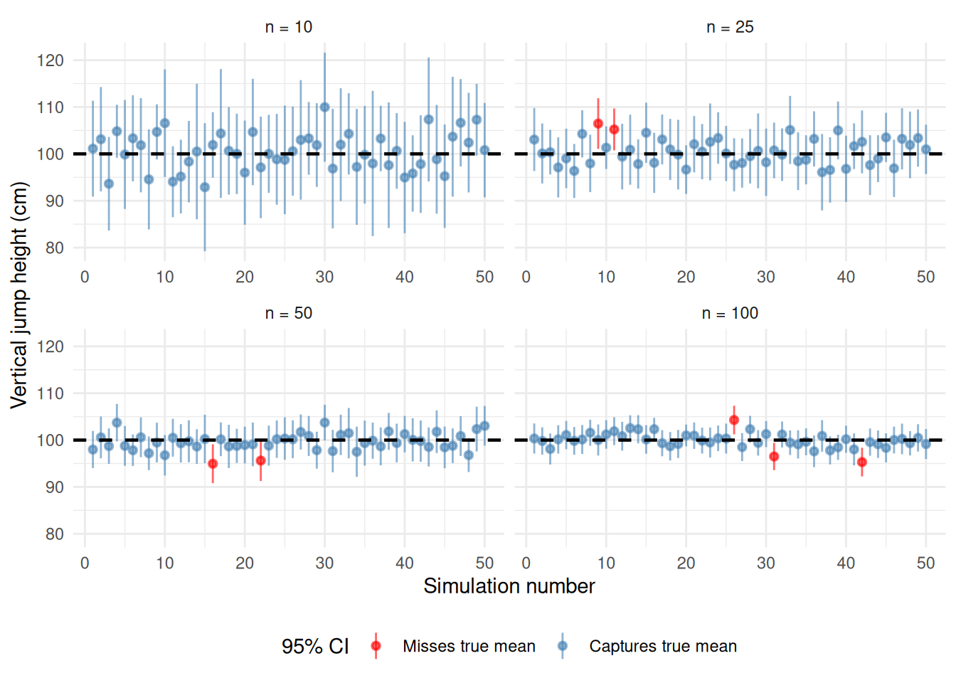
Figure 9.1: Effect of sample size on 95% confidence interval width. Larger samples produce narrower intervals, reflecting reduced sampling error. All samples drawn from a population with mean = 100 and SD = 15.
Figure Figure 9.1 illustrates how confidence interval width decreases as sample size increases. Each line represents one 95% confidence interval from a simulated sample. Notice that nearly 95% of intervals (blue) capture the true population mean (dashed line), while approximately 5% (red) miss it—exactly as expected[3,4]. Larger samples yield narrower intervals, providing more precise estimates of the population parameter[1].
9.5 Confidence intervals for mean differences
In Movement Science research, we often compare two groups or conditions (e.g., intervention vs. control, pre-test vs. post-test)[10,11]. Confidence intervals for mean differences quantify the uncertainty in the magnitude of the effect[4,14].
9.5.1 Independent samples (two-group comparison)
For independent groups (e.g., experimental group vs. control group), the 95% CI for the difference in means (\(\mu_1 - \mu_2\)) is:
If the confidence interval does not include zero, the difference is statistically significant at the chosen confidence level[2,4]. More importantly, the interval reveals the range of plausible effect sizes[14].
9.5.2 Paired samples (within-subject comparison)
For paired data (e.g., pre-post measurements on the same participants), compute the difference score for each participant (\(d_i = x_{i,\text{post}} - x_{i,\text{pre}}\)), then construct a CI for the mean difference[1]:
We are 95% confident that young adults have reaction times between 29.7 and 90.3 ms faster than older adults. Because zero is not in the interval, the difference is statistically significant[4]. The interval also indicates the minimum plausible effect size (29.7 ms), which may be important for assessing practical significance[11,14].
9.6 Confidence intervals and statistical significance
Confidence intervals provide an elegant way to assess statistical significance without relying solely on p-values[1,2].
9.6.1 The relationship between CIs and p-values
Key principle: If a 95% confidence interval for a difference does not include zero, the difference is statistically significant at \(\alpha = 0.05\) (two-tailed)[3,4].
Why? A 95% CI excludes values that are implausible at the 5% significance level. If zero (no effect) is outside the interval, we reject the null hypothesis of no difference[2,5].
TipAdvantages of confidence intervals over p-values
Effect size information: The interval reveals plausible magnitudes, not just “significant” vs. “not significant.”
Precision information: Narrow intervals indicate high precision; wide intervals indicate high uncertainty.
Clinical/practical relevance: Researchers can judge whether the entire interval falls within a range of practical importance.
Transparency: Intervals communicate uncertainty honestly rather than reducing findings to binary decisions.
9.6.2 Interpreting overlapping vs. non-overlapping confidence intervals
A common question: “If two 95% CIs overlap, does that mean there is no significant difference?”[4,20].
Answer: Not necessarily. Two groups can have overlapping 95% CIs yet still show a statistically significant difference when formally tested[20,21]. The correct comparison is to examine the confidence interval for the difference, not the overlap of individual group CIs[5].
Do not conclude “no significant difference” simply because two 95% CIs overlap. Instead, compute the 95% CI for the mean difference and check whether it includes zero[20,21].
9.7 Confidence intervals for proportions
Confidence intervals also apply to proportions (e.g., success rates, injury rates, adherence rates)[5,22].
For a sample proportion \(\hat{p} = x/n\) (where \(x\) is the number of successes), the approximate 95% CI is:
We are 95% confident that the true injury rate among recreational runners lies between 8.6% and 21.4%. The wide interval reflects the relatively small sample size and the inherent variability in injury occurrence[5,22].
9.8 Confidence intervals for effect sizes
Effect sizes (e.g., Cohen’s d, correlation coefficients) quantify the magnitude of effects in standardized units[1,14]. Like means and proportions, effect sizes carry uncertainty and should be reported with confidence intervals[6,13].
9.8.1 Cohen’s d with confidence intervals
Cohen’s d is defined as:
\[
d = \frac{\bar{x}_1 - \bar{x}_2}{s_{\text{pooled}}}
\]
Where \(s_{\text{pooled}}\) is the pooled standard deviation[14,24].
Computing exact confidence intervals for d requires specialized formulas or software (e.g., ESCI, R packages)[1,25]. The key insight: a confidence interval for d reveals the range of plausible standardized effect sizes, helping researchers assess both statistical and practical significance[13].
NoteReal example: Effect size with confidence
A meta-analysis reports that resistance training improves muscle strength with d = 0.67, 95% CI [0.52, 0.82]. Interpretation:
The best estimate of the standardized effect is moderate-to-large (d = 0.67)[24].
We are 95% confident the true effect is at least 0.52 (moderate) and at most 0.82 (large).
The narrow interval indicates high precision, likely due to a large meta-analytic sample[13,26].
9.9 Common misinterpretations of confidence intervals
Despite their utility, confidence intervals are frequently misinterpreted[15,16]. Avoid these errors:
9.9.1 Misinterpretation 1: “There is a 95% probability the true parameter is in this interval”
Correct interpretation: If we repeated the study infinitely many times and constructed a 95% CI each time, approximately 95% of those intervals would contain the true parameter[3,4]. The true parameter is fixed; the interval is random.
9.9.2 Misinterpretation 2: “Values outside the CI have been rejected”
Correct interpretation: Values outside the 95% CI are less plausible but not impossible[1]. The CI provides a range of values compatible with the data, not an absolute boundary[16].
9.9.3 Misinterpretation 3: “A 95% CI contains 95% of the sample data”
Correct interpretation: A confidence interval estimates the population parameter (e.g., the mean), not the distribution of individual observations[15]. To describe where most data fall, use prediction intervals or reference ranges[5].
ImportantUnderstanding what confidence intervals do and don’t tell you
Confidence intervals quantify uncertainty about a population parameter, not variability in individual observations[4,5]. A narrow CI means we have precisely estimated the population mean, but individuals may still vary widely around that mean.
9.10 Reporting confidence intervals
Best practices for reporting confidence intervals[1,6,27]:
Always report point estimates with CIs: “Mean VO₂max was 52.3 mL/kg/min, 95% CI [49.8, 54.8].”
Specify the confidence level: Make it clear whether you used 90%, 95%, or 99%.
Provide CIs for effect sizes: Report d = 0.67, 95% CI [0.52, 0.82], not just d = 0.67.
Interpret intervals in context: Discuss whether the interval width is acceptable for your research question[11].
Avoid overreliance on significance: Use CIs to assess practical importance, not just statistical significance[1,9].
9.11 Visualizing confidence intervals
Confidence intervals are often displayed graphically to facilitate interpretation[4,6].
9.11.1 Error bar plots
Error bars show means ± confidence intervals (or standard errors) for groups or conditions[1].
Code
library(ggplot2)# Simulated dataset.seed(456)groups <-c("Control", "Moderate Training", "Intensive Training")means <-c(380, 350, 320)se <-c(12, 10, 11)n <-c(20, 20, 20)# Compute 95% CIt_crit <-qt(0.975, df = n -1)ci_lower <- means - t_crit * seci_upper <- means + t_crit * sedf <-data.frame(Group =factor(groups, levels = groups),Mean = means,CI_lower = ci_lower,CI_upper = ci_upper)ggplot(df, aes(x = Group, y = Mean)) +geom_point(size =4, color ="steelblue") +geom_errorbar(aes(ymin = CI_lower, ymax = CI_upper), width =0.2, size =1, color ="steelblue") +labs(x ="Training Group", y ="Reaction Time (ms)", title ="Reaction Time by Training Group") +theme_minimal() +ylim(280, 420)
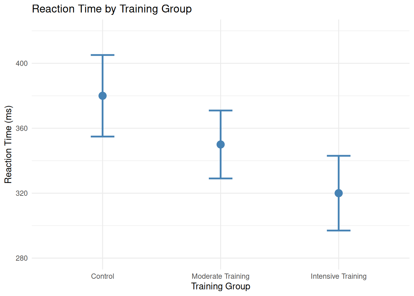
Figure 9.2: Mean reaction time (ms) with 95% confidence intervals for three training groups. Error bars that do not overlap suggest a significant difference, though formal testing is required.
Figure Figure 9.2 displays mean reaction times with 95% confidence intervals. The non-overlapping error bars suggest statistically significant differences between groups, particularly between Control and Intensive Training[4]. However, formal hypothesis testing or examination of the CI for the difference is required to confirm significance[20,21].
9.11.2 Forest plots for meta-analysis
In meta-analyses, forest plots display effect sizes and confidence intervals from multiple studies, along with the overall pooled estimate[13,26].
9.12 Sample size planning using confidence intervals
Confidence intervals are useful for sample size planning[1,17]. Researchers can determine the sample size needed to achieve a desired CI width, ensuring adequate precision[28].
General principle: To achieve narrower confidence intervals, increase sample size[3]. Software tools (e.g., G*Power, R packages) can compute required sample sizes for target CI widths[25,29].
TipPlanning for precision
Rather than focusing solely on “enough power to detect significance,” consider planning studies to achieve sufficiently narrow confidence intervals that provide informative estimates of effect magnitude[1,17]. This approach, called precision-based sample size planning, aligns with the goals of estimation and effect size reporting[28].
9.13 Chapter summary
Confidence intervals are indispensable tools for quantifying uncertainty and communicating research findings responsibly[1,6]. Unlike point estimates, which offer single numerical summaries, confidence intervals provide a range of plausible values for population parameters, acknowledging the inherent variability of sample-based estimates[2,5]. A 95% confidence interval means that if we repeated our study many times, approximately 95% of the intervals would capture the true population value—a property rooted in the logic of sampling distributions and the Central Limit Theorem[3,4]. Interval width is determined by sample size, data variability, and the chosen confidence level: larger samples, lower variability, and lower confidence levels produce narrower intervals[1].
Confidence intervals apply not only to means but also to mean differences, proportions, and effect sizes, making them versatile across diverse research contexts[13,14]. When a confidence interval for a difference does not include zero, the effect is statistically significant at the corresponding alpha level[4,5]. More importantly, confidence intervals reveal the magnitude and precision of effects, enabling researchers to assess practical significance alongside statistical significance[10,11]. By reporting “mean difference = 4.3 cm, 95% CI [2.1, 6.5],” researchers communicate both the best estimate and the range of uncertainty, fostering transparent and nuanced interpretation[6,27]. As Movement Science increasingly emphasizes effect sizes and open science, confidence intervals represent a shift from black-and-white dichotomous thinking to thoughtful, probabilistic reasoning about human performance data[1,9].
9.14 Key terms
confidence interval; point estimate; margin of error; critical value; standard error; confidence level; precision; mean difference; paired samples; independent samples; effect size; Cohen’s d; sampling error; statistical significance; practical significance
9.15 Practice: quick checks
Point estimates (e.g., sample mean) provide a single best guess of a population parameter but ignore uncertainty inherent in sampling[1]. Confidence intervals quantify that uncertainty by providing a range of plausible values, reflecting sampling variability[5]. For example, knowing that mean reaction time is 350 ms is useful, but knowing it is 350 ms, 95% CI [330, 370] tells us how precisely we have estimated it. Confidence intervals enable readers to judge both statistical and practical significance, fostering more honest and transparent communication of findings[4,6].
If a 95% confidence interval for a mean difference includes zero, it means zero is a plausible value for the true population difference[4]. In other words, the observed difference could be due to sampling variability alone, and we cannot confidently conclude that a true effect exists[2]. This corresponds to the difference being not statistically significant at \(\alpha = 0.05\) (two-tailed)[5]. However, including zero does not prove “no effect”; it simply means the data are consistent with no effect as well as with small positive or negative effects[1].
Increasing sample size narrows the confidence interval because it reduces sampling error[3]. The standard error decreases as \(1/\sqrt{n}\), so larger samples yield more precise estimates[1]. For instance, doubling the sample size reduces the standard error by approximately 30% (\(1/\sqrt{2} \approx 0.71\)). To cut the confidence interval width in half, you need to quadruple the sample size[17]. This principle is crucial for study planning: adequately powered studies with sufficient sample sizes provide narrower, more informative confidence intervals that better inform practice and policy[28].
Overlapping confidence intervals for individual group means do not directly test the difference between groups[20,21]. A formal comparison requires constructing a confidence interval for the difference (\(\bar{x}_1 - \bar{x}_2\)), which accounts for the correlation or pooled variability between groups[5]. Two groups can have overlapping 95% CIs yet produce a 95% CI for the difference that excludes zero, indicating statistical significance[4]. The correct approach is to compute the CI for the difference, not rely on visual overlap of group CIs[20]. This highlights the importance of appropriate statistical comparisons rather than informal “eyeball” tests.
Statistical significance refers to whether an effect is distinguishable from zero at a given alpha level (e.g., if the 95% CI excludes zero)[4]. Practical significance refers to whether the magnitude of the effect is large enough to matter in real-world contexts[11,14]. A confidence interval can exclude zero (statistically significant) but contain only trivially small effect sizes (not practically significant). Conversely, a wide interval might include zero (not statistically significant) yet also include large, practically important effects, warranting further research[1]. Researchers should evaluate both the location of the interval (does it exclude zero?) and its range (are plausible values practically meaningful?)[10].
A common misinterpretation is believing “there is a 95% probability that the true parameter lies within this specific interval”[15,16]. In frequentist statistics, the true parameter is fixed (though unknown), and the interval is random (varies across samples). The correct interpretation is: if we repeated the study infinitely and computed 95% CIs each time, approximately 95% of those intervals would capture the true parameter[3,4]. This is a statement about the long-run behavior of the method, not about the probability that any one interval contains the parameter[5]. Understanding this subtlety prevents overconfidence in individual intervals and promotes appropriate probabilistic reasoning.
NoteRead further
For deeper exploration of confidence intervals and their application to Movement Science research, see[1] (Understanding the New Statistics) and[5] (Statistics Notes series in BMJ). For effect size estimation and reporting, consult[14] and[13].
TipNext chapter
In Chapter 10, you will learn about hypothesis testing, the traditional framework for making yes/no decisions about research hypotheses. You will see how hypothesis tests relate to confidence intervals, understand Type I and Type II errors, and learn to interpret p-values responsibly in Movement Science research.
2. Gardner, M. J., & Altman, D. G. (1986). Confidence intervals rather than p values: Estimation rather than hypothesis testing. BMJ, 292(6522), 746–750. https://doi.org/10.1136/bmj.292.6522.746
3. Moore, D. S., McCabe, G. P., & Craig, B. A. (2021). Introduction to the practice of statistics (10th ed.). W. H. Freeman; Company.
4. Cumming, G. (2012). Understanding the new statistics: Effect sizes, confidence intervals, and meta-analysis. Routledge.
5. Altman, D. G., & Bland, J. M. (2000). Statistics notes: The use of transformation when comparing two means. BMJ, 312, 1153. https://doi.org/10.1136/bmj.312.7039.1153
6. Wilkinson, L., & Task Force on Statistical Inference. (1999). Statistical methods in psychology journals: Guidelines and explanations. American Psychologist, 54(8), 594–604. https://doi.org/10.1037/0003-066X.54.8.594
8. Schmidt, F. L. (1996). Statistical significance testing and cumulative knowledge in psychology: Implications for training of researchers. Psychological Methods, 1(2), 115–129. https://doi.org/10.1037/1082-989X.1.2.115
9. Kline, R. B. (2013). Beyond significance testing: Statistics reform in the behavioral sciences.
10. Hopkins, W. G., Marshall, S. W., Batterham, A. M., & Hanin, J. (2009). Progressive statistics for studies in sports medicine and exercise science. Medicine & Science in Sports & Exercise, 41(1), 3–13. https://doi.org/10.1249/MSS.0b013e31818cb278
11. Batterham, A. M., & Hopkins, W. G. (2006). Making meaningful inferences about magnitudes. International Journal of Sports Physiology and Performance, 1(1), 50–57. https://doi.org/10.1123/ijspp.1.1.50
12. Field, A. (2018). Discovering statistics using IBM SPSS statistics (5th ed.). SAGE Publications.
13. Nakagawa, S., & Cuthill, I. C. (2007). Effect size, confidence interval and statistical significance: A practical guide for biologists. Biological Reviews, 82, 591–605. https://doi.org/10.1111/j.1469-185X.2007.00027.x
14. Lakens, D. (2013). Calculating and reporting effect sizes to facilitate cumulative science: A practical primer for t-tests and ANOVAs. Frontiers in Psychology, 4, 863. https://doi.org/10.3389/fpsyg.2013.00863
15. Hoekstra, R., Morey, R. D., Rouder, J. N., & Wagenmakers, E.-J. (2014). Robust misinterpretation of confidence intervals. Psychonomic Bulletin & Review, 21, 1157–1164. https://doi.org/10.3758/s13423-013-0572-3
16. Morey, R. D., Hoekstra, R., Rouder, J. N., Lee, M. D., & Wagenmakers, E.-J. (2016). The fallacy of placing confidence in confidence intervals. Psychonomic Bulletin & Review, 23, 103–123. https://doi.org/10.3758/s13423-015-0947-8
17. Maxwell, S. E., Delaney, H. D., & Kelley, K. (2018). Designing experiments and analyzing data: A model comparison perspective (3rd ed.). Routledge.
18. Atkinson, G., & Nevill, A. M. (1998). Statistical methods for assessing measurement error (reliability) in variables relevant to sports medicine. Sports Medicine, 26(4), 217–238. https://doi.org/10.2165/00007256-199826040-00002
20. Schenker, N., & Gentleman, J. F. (2001). Judging statistical significance from confidence intervals. The American Statistician, 55(3), 182–186. https://doi.org/10.1198/000313001317098149
21. Cumming, G., & Finch, S. (2009). Inference by eye: Reading the overlap of independent confidence intervals. Statistics in Medicine, 28, 205–220. https://doi.org/10.1002/sim.3471
23. Agresti, A., & Coull, B. A. (1998). Approximate is better than "exact" for interval estimation of binomial proportions. The American Statistician, 52(2), 119–126. https://doi.org/10.1080/00031305.1998.10480550
24. Cohen, J. (1988). Statistical power analysis for the behavioral sciences (2nd ed.). Lawrence Erlbaum Associates.
25. Kelley, K., & Preacher, K. J. (2012). On effect size. Psychological Methods, 17(2), 137–152. https://doi.org/10.1037/a0028086
26. Borenstein, M., Hedges, L. V., Higgins, J. P. T., & Rothstein, H. R. (2009). Introduction to meta-analysis. John Wiley & Sons.
27. American Psychological Association. (2020). Publication manual of the american psychological association (7th ed.). American Psychological Association.
28. Kelley, K. (2007). Sample size planning for the coefficient of variation from the accuracy in parameter estimation approach. Behavior Research Methods, 39(4), 755–766. https://doi.org/10.3758/BF03192966
29. Faul, F., Erdfelder, E., Lang, A.-G., & Buchner, A. (2007). G*power 3: A flexible statistical power analysis program for the social, behavioral, and biomedical sciences. Behavior Research Methods, 39(2), 175–191. https://doi.org/10.3758/BF03193146