Locating individual performance within a group and across different scales
Tip💻 SPSS Tutorial Available
Learn how to calculate percentiles and standard scores in SPSS! See the SPSS Tutorial: Percentiles and Z-Scores in the appendix for step-by-step instructions on computing percentile ranks, z-scores, and interpreting standardized values in performance assessment contexts.
6.1 Chapter roadmap
Describing distributions with measures of center and spread tells you about the group as a whole. But in Movement Science practice, you often need to answer a different question: where does this individual stand relative to others? When an athlete produces a vertical jump height of 45 cm, is that typical, below average, or exceptional? When a patient scores 72 on a balance assessment, how does that compare to age-matched norms? When you want to compare an athlete’s sprint time to their flexibility score, how do you account for the fact that these measurements use completely different scales and units? These questions require tools that locate individual values within distributions and, when needed, transform different measurements onto a common scale for meaningful comparison[1].
Percentiles answer the location question by telling you what percentage of the distribution falls at or below a given value. A percentile rank of 75 means the individual performed as well as or better than 75 percent of the comparison group. Percentiles are especially useful in Movement Science because they are scale-free (they work equally well for sprint times, strength scores, and flexibility measures), resistant to outliers, and immediately interpretable without making distributional assumptions[1]. They are the foundation of normative databases in fitness testing, clinical assessments, and talent identification contexts. However, percentiles have limitations: equal percentile differences do not represent equal performance differences, percentile ranks can be unstable in small samples, and they do not preserve the metric properties needed for many statistical operations[1].
Standard scores, particularly z-scores, address different needs by expressing how many standard deviations an observation falls from the mean. A z-score of +2.0 indicates performance two standard deviations above the mean, regardless of whether you are measuring sprint time, grip strength, or VO₂max. This transformation creates a common scale that enables cross-variable comparisons, supports identification of unusual values, and connects directly to probability statements when distributions are approximately normal[1]. In Movement Science, z-scores and related transformations are used in talent identification batteries, return-to-play assessments, multi-component fitness evaluations, and research contexts where you need to combine or compare measures with different units. The key limitation is that z-scores perform best when distributions are roughly symmetric and unimodal; with strong skew or outliers, z-scores can be misleading because they depend on the mean and standard deviation, which are themselves sensitive to distributional shape[1].
By the end of this chapter, you will be able to:
Compute and interpret percentiles and percentile ranks for individual observations.
Explain common percentile divisions (quartiles, quintiles, deciles) and their uses in Movement Science.
Calculate and interpret z-scores and other standard scores.
Compare observations across different measurement scales using standardization.
Recognize when percentiles are more appropriate than z-scores and vice versa.
Apply these tools to fitness testing, clinical assessment, and talent identification contexts.
6.2 Workflow used throughout this chapter
Use this sequence when locating individual performance within a group:
Identify the reference distribution (norms, baseline sample, or comparison group).
Decide between percentile-based or standard score approaches based on distribution shape and purpose.
Compute the location measure (percentile rank or z-score).
Interpret the result in context (what does this mean for this individual?).
Consider measurement error and sample size when making judgments.
6.3 Why individual location matters in Movement Science
Much of Movement Science practice involves comparing individuals to reference standards. Fitness professionals assess cardiovascular endurance against age and sex norms. Physical therapists track balance scores relative to fall-risk cutoffs. Sport scientists evaluate an athlete’s sprint time against team benchmarks or talent identification criteria. In each case, the raw score alone is insufficient; you need context to know whether 3.45 seconds is fast, average, or slow for this group[1].
Location measures provide that context in two complementary ways. Percentiles rank individuals within a distribution, answering “how does this person compare to others?” without requiring any assumption about the shape of the distribution. Standard scores quantify distance from the mean in standard deviation units, answering “how unusual is this value?” in a way that connects to probability and enables cross-scale comparisons. Choosing between them (or using both) depends on your distribution, your question, and your purpose.
A practical example clarifies the difference. Suppose two athletes are evaluated on sprint time and vertical jump:
Athlete A: sprint = 3.20 s (z = −1.5), vertical jump = 50 cm (z = +1.2)
Athlete B: sprint = 3.30 s (z = −0.8), vertical jump = 48 cm (z = +0.8)
The z-scores immediately reveal that Athlete A shows greater strength (higher jump) but also faster speed (lower time = more negative z for a “lower is better” measure). Without standardization, comparing 3.20 s to 50 cm is meaningless because the units differ. With z-scores, you can see that both athletes have strengths, but Athlete A shows more extreme deviation from the mean in both directions.
NoteReal example: normative fitness databases
Many fitness testing batteries report percentile ranks based on age and sex. For example, a 20-year-old female with a 1-mile run time at the 60th percentile is faster than 60 percent of women in that age group. Over time, as she ages, her raw time might stay the same, but her percentile rank could change because the reference group changes. This highlights that percentile ranks are always relative to a defined comparison group.
6.4 Percentiles and percentile ranks
6.4.1 What is a percentile?
The pth percentile is the value at or below which p percent of the distribution falls[1]. For example, the 25th percentile (also called the first quartile, Q₁) is the value that separates the lowest 25 percent from the upper 75 percent. The 50th percentile is the median. The 75th percentile (Q₃) separates the lowest 75 percent from the upper 25 percent.
A percentile rank answers the reverse question: given a specific value, what percentage of the distribution is at or below it? If an athlete’s sprint time corresponds to the 80th percentile, that athlete is faster than 80 percent of the comparison group (assuming lower times are better).
Important: percentiles and percentile ranks are not the same thing, though they are closely related. A percentile is a location on the scale (a value), while a percentile rank is a percentage (how much of the data is below that value).
6.4.2 Computing percentiles by hand
For small datasets, percentiles can be computed by sorting the data and finding the position that corresponds to the desired percentage. Different methods exist, and software packages may use slightly different conventions, but the logic is the same: locate the position in the ordered data that divides it at the target proportion[1].
One common method uses the formula:
\[
L = \frac{p}{100}(n+1)
\]
where L is the location in the ordered dataset and p is the desired percentile. If L is a whole number, the percentile is the value at that position. If L is fractional, interpolate between the two surrounding values.
6.4.2.1 Worked example: computing the 30th percentile
Use this dataset of 10 sprint times (in seconds), unsorted:
Approximately 30 percent of sprint times in this sample are at or below 3.413 seconds. If an athlete runs 3.40 seconds, they are performing slightly better than the 30th percentile benchmark for this group.
WarningCommon mistake
Confusing the percentile (a value on the measurement scale) with the percentile rank (a percentage). The 30th percentile is 3.413 seconds. If someone asks “what is the percentile rank of 3.40 seconds?” you would say “slightly below the 30th percentile,” not “3.40th percentile.”
6.4.3 Computing percentile ranks
Given an individual’s score, the percentile rank estimates what percentage of the distribution falls at or below that score. A simple method for small samples is:
This athlete’s sprint time is at approximately the 60th percentile, meaning they performed as well as or better than 60 percent of the sample. In “lower is better” scales like sprint time, a higher percentile rank indicates better performance (faster time).
6.4.4 Percentiles are resistant
Percentiles depend only on rank order, not on the magnitude of extreme values. This makes them highly resistant to outliers and skew. If the slowest sprint time changes from 3.55 to 4.00 seconds, the 30th percentile does not change at all because it depends only on the sorted positions, not on how far apart the values are[1].
This resistance is valuable in Movement Science contexts where distributions can be skewed (e.g., reaction time, sway area) or where occasional unusual values occur (equipment error, participant distraction).
6.4.5 Visualizing percentiles
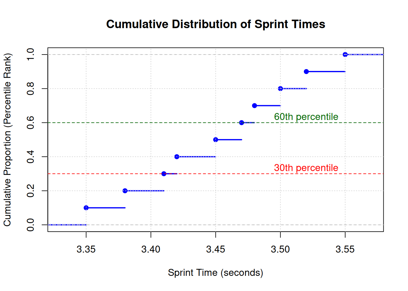
A cumulative distribution function (CDF) shows percentile ranks directly. The y-axis represents the cumulative proportion (percentile rank as a decimal), and the x-axis represents the measurement scale.
Code
# Sprint times from worked examplesprint_times <-c(3.35, 3.38, 3.41, 3.42, 3.45, 3.47, 3.48, 3.50, 3.52, 3.55)# Create empirical CDFplot(ecdf(sprint_times), main ="Cumulative Distribution of Sprint Times", xlab ="Sprint Time (seconds)", ylab ="Cumulative Proportion (Percentile Rank)",col ="blue", lwd =2)grid()# Highlight 30th and 60th percentilesabline(h =0.30, col ="red", lty =2)abline(h =0.60, col ="darkgreen", lty =2)text(3.52, 0.33, "30th percentile", col ="red")text(3.52, 0.63, "60th percentile", col ="darkgreen")
Figure 6.1: Cumulative distribution function showing percentile ranks for sprint times
This cumulative distribution function (CDF) provides a visual representation of percentile ranks across the entire sprint time distribution. The step-like pattern reflects the discrete nature of the small sample (n=10). To find the percentile rank of any value, locate it on the x-axis and read up to the curve, then across to the y-axis. For example, the value 3.47 seconds corresponds to approximately 0.60 (60th percentile), meaning 60% of the sample had sprint times at or below this value. The red and green dashed lines highlight the 30th and 60th percentiles respectively, illustrating how different performance levels map onto the distribution. With larger samples, the step pattern smooths into a continuous curve, making percentile estimation more precise.
6.5 Common percentile divisions
Percentiles can be grouped into divisions that provide useful benchmarks for interpretation:
6.5.1 Quartiles
Quartiles divide the distribution into four equal parts[1]:
Q₁ (25th percentile): 25% of values fall below this point
Q₂ (50th percentile): the median
Q₃ (75th percentile): 75% of values fall below this point
The interquartile range (IQR = Q₃ − Q₁) contains the middle 50% of observations. Quartiles are commonly used in box plots and as robust summaries of spread.
6.5.2 Quintiles
Quintiles divide the distribution into five equal parts (20th, 40th, 60th, 80th percentiles). These are sometimes used in talent identification contexts to classify athletes into performance bands (e.g., top 20%, next 20%, etc.).
6.5.3 Deciles
Deciles divide the distribution into ten equal parts (10th, 20th, …, 90th percentiles). Deciles provide finer resolution for classification. For example, a fitness test might report results in decile bands to give more granular feedback than quartiles provide.
6.5.4 Percentile-based classifications in Movement Science
Many Movement Science applications use percentile cutoffs to define categories:
Fitness testing: VO₂max standards often report values by quintiles or deciles for age and sex groups.
Clinical assessment: Balance scores may define fall-risk categories based on percentile cutoffs (e.g., below the 10th percentile = high risk).
Talent identification: Young athletes may be classified as “emerging” (above 75th percentile) or “elite” (above 90th percentile) for their age group.
Return-to-play: Symmetry indices or performance scores may need to reach the 50th percentile of pre-injury norms before clearance.
NoteReal example: physical fitness test battery
A common fitness battery might report:
Cardiovascular endurance (1-mile run time): 75th percentile (good)
Each component is evaluated against age and sex norms. The percentile ranks allow comparison across components despite different units and scales. A coach can see that this individual has relative strength in aerobic fitness and relative weakness in flexibility, guiding targeted training interventions.
6.6 Z-scores and standardization
6.6.1 What is a z-score?
A z-score (also called a standard score) expresses how many standard deviations an observation falls from the mean[1]:
\[
z = \frac{x - \bar{x}}{s}
\]
where:
\(x\) = individual’s raw score
\(\bar{x}\) = sample mean
\(s\) = sample standard deviation
A z-score of 0 means the value equals the mean. A z-score of +1 means the value is one standard deviation above the mean. A z-score of −2 means the value is two standard deviations below the mean.
6.6.2 Interpreting z-scores
Z-scores tell you about location and unusualness:
Typical values: z-scores between −1 and +1 are considered within one standard deviation of the mean, which captures roughly 68% of data in a normal distribution.
Moderately unusual: z-scores between ±1 and ±2 represent moderate departures from the mean.
Unusual: z-scores beyond ±2 or ±3 represent increasingly rare values in normal distributions.
However, these interpretations assume an approximately normal distribution. For skewed or bounded distributions, z-scores can be computed algebraically, but their interpretation as “unusual” depends on the distributional context[1].
ImportantCritical point about z-scores
Z-scores standardize the mean and standard deviation, so they perform best when the distribution is roughly symmetric and unimodal. For skewed distributions, z-scores can still be computed, but extreme values inflate the standard deviation, and mean-based distances may not correspond to intuitive notions of “typical” or “unusual.” In such cases, percentile ranks often provide more faithful summaries.
6.6.3 Worked example: computing z-scores
Use the sprint time dataset with mean and standard deviation:
Interpretation: Athlete A is 1.61 standard deviations faster than the mean (negative z-score indicates lower time, which is better in sprint contexts).
Interpretation: Athlete C’s time is essentially at the mean (z ≈ 0), indicating average performance for this group.
6.6.4 Properties of z-scores
Z-scores have mathematically useful properties that make them valuable for further analysis:
Standardized scale: Z-scores always have a mean of 0 and a standard deviation of 1, regardless of the original units.
Linear transformation: Z-scores preserve the shape of the distribution. If the raw data are skewed, the z-scores will be skewed in the same way.
Unit-free comparison: Z-scores enable comparison across different measurement scales because they express location in standard deviation units rather than raw units.
Outlier identification: Values with z-scores beyond ±2 or ±3 are often flagged as potential outliers, though this rule works best for symmetric distributions[1].
6.6.5 Comparing performance across different tests using z-scores
Z-scores are especially useful when you need to compare performance on tests with different units. This is common in multi-component fitness batteries, return-to-play evaluations, and talent identification.
6.6.5.1 Worked example: cross-test comparison
An athlete completes three tests with the following results and group norms:
(Below average; negative because lower reach is worse)
Interpretation
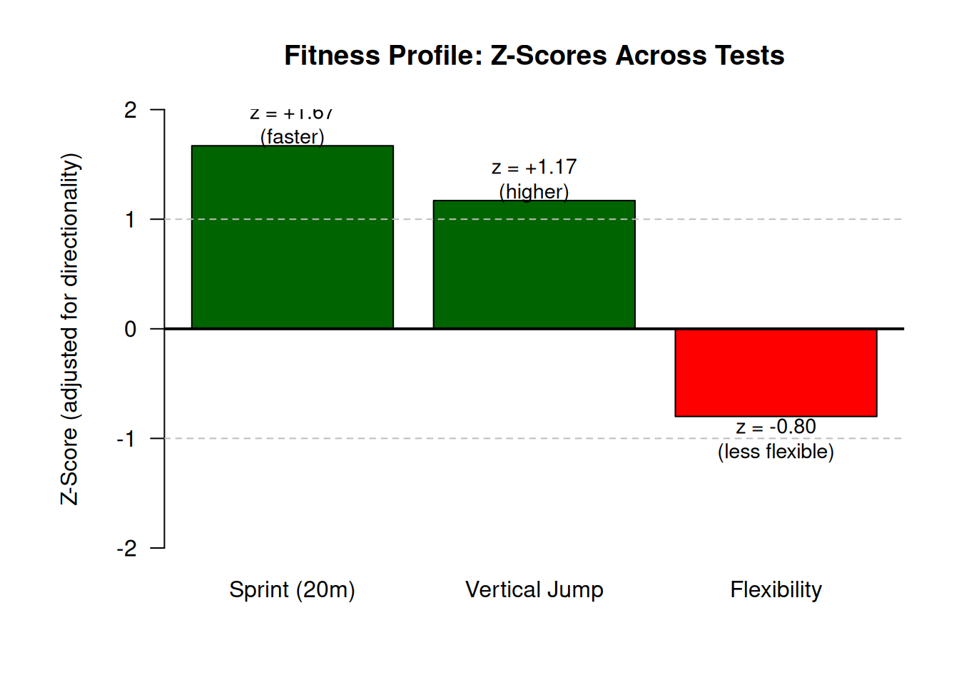
The athlete shows relative strength in sprint speed (z = −1.67, well below mean time) and vertical jump (z = +1.17, above mean height), but relative weakness in flexibility (z = −0.80, below mean reach). The z-scores place all three performances on a common scale, making it easy to see where strengths and deficits lie. This pattern might suggest training priorities: maintaining power and speed while improving flexibility.
Code
# Z-scores for the three teststests <-c("Sprint (20m)", "Vertical Jump", "Flexibility")z_scores <-c(-1.67, 1.17, -0.80)# Adjust z-scores for "lower is better" tests to make interpretation clearer# For sprint, we'll plot the absolute value with "better" being positivez_scores_adjusted <-c(1.67, 1.17, -0.80)# Create bar plotpar(mar =c(5, 6, 4, 2))barplot(z_scores_adjusted, names.arg = tests, col =ifelse(z_scores_adjusted >0, "darkgreen", "red"),ylim =c(-2, 2),ylab ="Z-Score (adjusted for directionality)",main ="Fitness Profile: Z-Scores Across Tests",border ="black", las =1)abline(h =0, lwd =2)abline(h =c(-1, 1), lty =2, col ="gray")text(x =c(0.7, 1.9, 3.1), y = z_scores_adjusted +sign(z_scores_adjusted)*0.2, labels =c("z = +1.67\n(faster)", "z = +1.17\n(higher)", "z = -0.80\n(less flexible)"),cex =0.9)
Figure 6.2: Z-score profile across three fitness tests showing relative strengths and weaknesses
This z-score profile visualizes the athlete’s relative performance across three fitness components. Positive bars (green) indicate above-average performance, while negative bars (red) indicate below-average performance, with all values adjusted so that “up” means “better” regardless of the raw test’s directionality. The athlete shows notable strength in sprint speed (z = +1.67, meaning 1.67 SD faster than average) and vertical jump (z = +1.17, meaning 1.17 SD higher than average), but a relative weakness in flexibility (z = −0.80, meaning 0.80 SD less flexible than average). The dashed horizontal lines at ±1 represent one standard deviation from the mean, a common threshold for identifying moderate departures from typical performance. This type of profile is valuable in Movement Science for identifying training priorities, monitoring balanced development, and making talent identification decisions based on multi-component assessments.
6.7 Other standard scores
While z-scores have a mean of 0 and standard deviation of 1, other standard scores are linear transformations designed for convenience or tradition in specific contexts.
6.7.1 T-scores
T-scores are transformed z-scores with a mean of 50 and standard deviation of 10:
\[
T = 10z + 50
\]
T-scores avoid negative numbers and decimals, which can be easier to communicate in applied settings. A T-score of 40 corresponds to z = −1 (one SD below the mean), while a T-score of 60 corresponds to z = +1.
6.7.2 Other linear transformations
Many standardized tests use similar transformations:
IQ scores: mean = 100, SD = 15
SAT scores (historically): mean = 500, SD = 100
Stanines: 1–9 scale with mean ≈ 5, SD ≈ 2 (discrete categories)
These are all linear transformations of z-scores, so they preserve the shape of the distribution and the relative distances between observations. The only difference is the scale for reporting[1].
6.7.2.1 Worked example: converting z-score to T-score
From the earlier sprint example, Athlete A had z = −1.61.
Convert to T-score:
\[
T = 10(-1.61) + 50 = -16.1 + 50 = 33.9
\]
Interpretation
A T-score of 33.9 indicates performance 1.61 standard deviations below the mean, expressed on a scale where 50 is average and each 10-point change represents one standard deviation. This scale avoids negative numbers and may be preferable in some reporting contexts.
6.8 Percentiles vs. z-scores: when to use which
Both percentiles and z-scores locate individuals within distributions, but they have different strengths and limitations. Choosing the appropriate tool depends on the distribution’s shape, the purpose of the comparison, and the statistical operations you need to perform.
Feature
Percentiles
Z-Scores
Assumption about distribution
None (nonparametric)
Best for symmetric, unimodal distributions
Resistance to outliers
Highly resistant
Sensitive (uses mean and SD)
Ease of interpretation
Intuitive (“better than X%”)
Requires understanding of SDs
Cross-scale comparison
Not directly comparable
Directly comparable (common scale)
Connection to probability
Direct (percentile = cumulative %)
Strong if distribution is normal
Use in further statistics
Limited
Widely used in inferential methods
Best for skewed data
Yes
No (can mislead)
6.8.1 When percentiles are preferred
The distribution is skewed or has outliers.
The measurement scale is ordinal (e.g., Likert scales, pain ratings).
You need a simple, intuitive summary for applied audiences.
You are creating normative categories (e.g., fitness percentile bands).
Sample size is small and distributional assumptions are uncertain.
6.8.2 When z-scores are preferred
The distribution is roughly symmetric and unimodal.
You need to compare scores across different measurement scales.
You are performing further statistical analyses that assume normality.
You want to identify outliers systematically (e.g., values with |z| > 3).
You need to connect individual performance to probability (via the normal curve, covered in Chapter 7).
6.8.3 Using both
In practice, reporting both percentile ranks and z-scores can provide complementary information. For example:
Sprint time: 3.35 s (60th percentile, z = −1.61)
This tells the reader that the performance is faster than 60% of the group and 1.61 standard deviations below the mean. If the distribution is roughly symmetric, these interpretations align well. If the distribution is skewed, the percentile may be more trustworthy.
NoteReal example: return-to-play assessment
A physical therapist assesses a patient’s balance after ankle surgery. The patient scores 45 on a balance test. Reference data show:
Mean = 50, SD = 8 → z = (45 − 50) / 8 = −0.63
Percentile rank ≈ 26th percentile
The z-score indicates performance is about two-thirds of a standard deviation below the mean—not extreme, but below average. The percentile rank indicates the patient scored better than only 26% of the reference group. Together, these suggest the patient has not fully recovered to typical levels, supporting a decision to continue rehabilitation before clearance for full activity.
6.9 Applied examples in Movement Science
6.9.1 Fitness testing and normative databases
Fitness test batteries commonly report results using percentile ranks based on large normative samples stratified by age and sex. For example:
Cardiovascular endurance: 1-mile run time → 70th percentile for 20-year-old females
Muscular strength: Push-ups to fatigue → 55th percentile
Body composition: Body fat percentage → 40th percentile
These percentile ranks provide immediate context: “This individual is above average in cardiovascular fitness, about average in strength, and slightly below average in body composition relative to peers.” Fitness professionals use these profiles to design individualized training programs that target relative weaknesses while maintaining strengths.
6.9.2 Clinical assessment and fall risk
Balance and mobility assessments often use percentile cutoffs to stratify risk. For example, the Berg Balance Scale or Timed Up and Go (TUG) test may define:
Low risk: Above 50th percentile
Moderate risk: 25th–50th percentile
High risk: Below 25th percentile
Patients below critical thresholds receive targeted interventions (balance training, assistive devices, home modifications). The percentile framework allows clinicians to communicate risk in accessible terms and track improvement over time by monitoring changes in percentile rank.
6.9.3 Talent identification in youth sport
Talent identification programs often assess young athletes across multiple physical, technical, and cognitive domains. Z-scores enable comparison across domains with different scales (e.g., sprint time in seconds, jump height in centimeters, agility score as a composite). Coaches can create composite scores by averaging z-scores across tests, identifying athletes who excel in multiple areas.
For example, a talent identification battery might include:
An athlete with a composite z-score above +1.0 might be classified as “emerging talent,” while those above +1.5 might be flagged as “elite prospects” for further development. This standardization ensures that tests with different units contribute equally to the composite.
6.9.4 Return-to-sport decision-making
Return-to-sport protocols often require athletes to meet multiple benchmarks before clearance. These may include:
Strength symmetry: <10% difference between limbs (z-scores can compare injured vs. uninjured limb relative to norms)
Functional performance: Performance on hop tests must reach ≥90% of pre-injury levels or ≥50th percentile of normative data
Patient-reported outcomes: Symptom scores below a critical percentile threshold
By combining z-scores and percentile ranks across domains, clinicians make evidence-based decisions that balance objective performance with patient-reported function.
6.10 Limitations and cautions
6.10.1 Sample size and stability
Both percentiles and z-scores can be unstable in small samples. A single extreme value can shift percentile ranks noticeably, and the sample mean and SD (used for z-scores) are themselves estimates with sampling variability. With very small samples (n < 20), treat extreme percentile ranks (e.g., 5th or 95th) and extreme z-scores (|z| > 2) with caution, as they may not replicate well in repeated testing[1].
6.10.2 Measurement error
All measurements contain error. An athlete who scores at the 60th percentile today might score at the 55th or 65th percentile tomorrow due to normal fluctuations in performance and measurement noise. Similarly, a z-score of +1.0 might shift to +0.8 or +1.2 on retesting. Interpret individual scores within the context of expected measurement variability (see Chapter 18 on reliability for more detail)[2].
6.10.3 Normative data currency
Percentile ranks are only as good as the normative database. If norms are outdated (e.g., based on data from 20 years ago) or unrepresentative (e.g., based on college athletes when assessing recreational participants), the percentile ranks may mislead. Always verify that the reference group matches the population of interest in terms of age, sex, training status, and other relevant characteristics.
6.10.4 Conflating percentile and percentage correct
In cognitive testing or skill assessments, a “percentage correct” (e.g., 80% of questions answered correctly) is not the same as a percentile rank (better than 80% of test-takers). These are easily confused, and the distinction matters. A student who scores 80% correct might be at the 90th percentile if the test is hard, or the 50th percentile if the test is easy. Always clarify which meaning is intended.
WarningCommon mistake
Interpreting all distributions as normal and assuming that z = +2 always means “better than 95% of people.” This is only true if the distribution is approximately normal. For skewed distributions, z-scores can still be computed, but their connection to percentiles changes. Always check distributional shape before interpreting z-scores probabilistically.
6.11 Worked example using the Core Dataset
This section demonstrates practical application using a realistic Movement Science scenario.
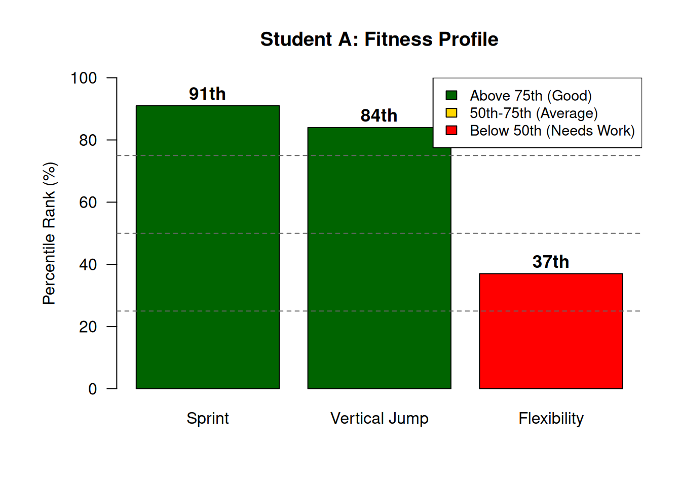
Sprint z = −1.33 → approximately 9th percentile in raw time, but 91st percentile in performance (faster than 91% of peers, because lower time is better).
Vertical Jump z = +1.00 → approximately 84th percentile (higher than 84% of peers).
Flexibility z = −0.33 → approximately 37th percentile (better than only 37% of peers).
Step 4: Create a profile and recommendations
Strengths: Sprint speed and vertical jump (both > 80th percentile) Relative weakness: Flexibility (37th percentile) Recommendation: Maintain power-based training; add regular flexibility work to improve range of motion and reduce injury risk.
This example illustrates how z-scores and percentile ranks work together to provide a comprehensive performance profile. The standardization allows direct comparison across tests with different units, while the percentile ranks make the results accessible to non-technical audiences.
Figure 6.3: Fitness profile for Student A showing percentile ranks across three components
This fitness profile visualizes Student A’s relative standing across three fitness components using percentile ranks, which are more intuitive for applied audiences than z-scores. Green bars indicate strong performance (above 75th percentile), gold indicates average performance (50th–75th), and red indicates areas needing improvement (below 50th). The dashed horizontal lines at the 25th, 50th, and 75th percentiles provide reference points for interpretation. Student A shows clear strengths in sprint speed (91st percentile) and vertical jump (84th percentile), both power-related attributes, but demonstrates a relative weakness in flexibility (37th percentile). This type of profile is widely used in fitness centers, sports medicine clinics, and talent identification programs to communicate results to athletes, clients, and coaches in an accessible format.
6.12 Chapter summary
Percentiles and standard scores are essential tools for locating individual performance within a group and enabling comparisons across different measurement scales[1]. Percentiles express the proportion of the distribution at or below a given value and are highly resistant to outliers and skew, making them ideal for normative databases, clinical cutoffs, and fitness classifications where distributions may be non-normal. Percentile ranks are intuitive and accessible, but they do not preserve equal intervals and cannot be directly manipulated in many statistical procedures[1]. Z-scores standardize observations by expressing them as deviations from the mean in standard deviation units, creating a common scale that enables cross-test comparisons and connects to probability when distributions are approximately normal. However, z-scores depend on the mean and standard deviation, so they are sensitive to outliers and perform best with roughly symmetric distributions[1]. In Movement Science applications, including fitness testing, clinical assessment, talent identification, and return-to-sport decisions, choosing between percentiles and z-scores (or using both) depends on distributional shape, the audience, and the scientific purpose. Understanding both approaches allows practitioners to communicate individual performance relative to norms in ways that are statistically sound and practically meaningful[2].
6.13 Key terms
percentile; percentile rank; quartile; quintile; decile; interquartile range; z-score; standard score; standardization; T-score; normative data; cumulative distribution function; linear transformation; outlier identification; cross-scale comparison
6.14 Practice: quick checks
A 30th percentile score means the patient performed as well as or better than 30 percent of the reference group, or equivalently, 70 percent of the reference group scored higher. Whether this is concerning depends on the clinical context and the reference group. If the test is used to stratify fall risk and scores below the 25th percentile indicate high risk, then the 30th percentile is just above the high-risk threshold. However, it still represents below-average performance and may warrant monitoring or targeted intervention. Always interpret percentile ranks relative to clinically meaningful cutoffs and consider measurement error—a score at the 30th percentile could easily be 25th or 35th on repeated testing.
A z-score of +2.5 indicates the athlete’s vertical jump is 2.5 standard deviations above the mean for the reference group. This is an unusually high value, representing exceptional performance. If the distribution is approximately normal, a z-score of +2.5 corresponds to roughly the 99th percentile, meaning the athlete jumps higher than approximately 99 percent of the comparison group. This level of performance would typically be classified as elite or outlier status, depending on the context. It suggests this athlete has notable lower-body power that may be worth leveraging in sport-specific training or talent identification programs.
Comparing 3.25 seconds to 35 centimeters is meaningless because the measurements use completely different units and scales—there is no basis for saying one is “better” or “worse” than the other. Z-scores solve this by transforming both values into a common scale: standard deviations from the mean. If the sprint time has a z-score of −1.8 (1.8 SD faster than average) and the sit-and-reach has a z-score of +0.5 (0.5 SD more flexible than average), we can now see that the athlete shows greater relative strength in sprint speed than in flexibility. The z-scores remove the dependency on units and allow direct comparison of relative standing within each domain.
Percentiles are preferable when the distribution is skewed or contains outliers, when the measurement scale is ordinal, when the audience needs intuitive summaries (e.g., “better than 75% of peers”), or when creating normative categories for applied use (e.g., fitness test bands). Percentiles make no assumptions about distributional shape and are highly resistant to extreme values. Z-scores are preferable when the distribution is roughly symmetric and unimodal, when you need to compare performance across different measurement scales, when performing further statistical analyses that assume normality, or when you want to identify outliers systematically (e.g., flagging values with |z| > 3). If both conditions are met, reporting both provides complementary information: percentile ranks for accessibility and z-scores for standardization.
Norms from 2000 may no longer accurately represent the current population due to secular trends—systematic changes over time in physical fitness, body composition, and health status. For example, if obesity rates have increased and physical activity has decreased since 2000, average fitness scores may have declined, meaning current clients might receive inflated percentile ranks (appearing “better” relative to an outdated norm). Conversely, if performance standards have improved (e.g., due to better training methods), current clients might receive deflated ranks. Additionally, norms may not match the demographics or training status of current clients. Always verify that normative data are recent (within 5–10 years), representative of the target population, and collected using the same testing protocols.
T-scores have a mean of 50 and a standard deviation of 10, so a T-score of 48 corresponds to a z-score of −0.2 (calculated as (48 − 50) / 10 = −0.2). This indicates performance is 0.2 standard deviations below the mean, which is very close to average. In practical terms, this athlete’s performance is essentially typical for the reference group, with no meaningful deviation in either direction. T-scores are often used in standardized testing contexts because they avoid negative numbers and decimals, making results easier to communicate to non-technical audiences.
NoteRead further
For applied perspectives on normative data and individual assessment in sport and exercise contexts, see discussions of measurement and interpretation in fitness testing manuals and sports medicine texts. For a statistical foundation on percentiles and z-scores, see introductory statistics texts such as[1]. For Movement Science-specific applications in reliability and measurement, see[2] and[3].
TipNext chapter
The next chapter introduces the normal distribution and its properties, connecting z-scores to probability statements and explaining when and why the normal curve is a useful model for Movement Science data.
1. Moore, D. S., McCabe, G. P., & Craig, B. A. (2021). Introduction to the practice of statistics (10th ed.). W. H. Freeman; Company.