Analyzing main effects, interactions, and mixed designs in Movement Science
Tip💻 Analytical Software & SPSS Tutorials
A Note on By-Hand Calculations: The purpose of this book is not to teach tedious by-hand statistical calculations. Modern researchers run these analyses using major software packages. While we provide the underlying equations for conceptual understanding, we strongly recommend relying on software for computation to avoid errors and save time.
Please direct your attention to the SPSS Tutorial: Factorial ANOVA in the appendix for step-by-step instructions on running both between-subjects and mixed factorial ANOVAs, interpreting interaction plots, conducting simple effects analysis, and computing effect sizes!
16.1 Chapter roadmap
The between-subjects ANOVA introduced in Chapter 14 answered one question at a time: does the training program affect strength? Does group membership predict aerobic capacity? These are clean, elegant questions — but they are also incomplete descriptions of how human movement and performance actually work. In practice, a researcher interested in resistance training does not simply ask whether training improves strength. She asks who benefits, by how much, and when the gains emerge. These questions involve at least two independent variables acting simultaneously, and the statistical tool required to address them is the factorial ANOVA.
A factorial design is one in which the researcher manipulates or observes two or more independent variables — called factors — simultaneously and examines their individual and combined effects on a single outcome variable. The power of the factorial approach lies in the word combined: beyond estimating the effect of each factor in isolation (the main effects), the factorial ANOVA tests whether the effect of one factor depends on the level of another. This conditional relationship is called an interaction, and interactions are among the most scientifically interesting findings in all of movement science research. A training program that improves strength in male athletes but not female athletes, or that produces gains in the first training block but not the second, involves an interaction — and a factorial design is required to detect it[1,2].
This chapter develops the factorial ANOVA framework across three design types that movement science researchers commonly encounter. The between-subjects factorial ANOVA (also called two-way ANOVA) tests the effects of two or more between-groups factors, where each participant appears in only one combination of factor levels. The mixed factorial ANOVA — arguably the most common design in training and rehabilitation research — combines at least one between-subjects factor (such as group) with at least one within-subjects (repeated measures) factor (such as time), allowing the researcher to ask whether groups differ in how they change. The within-within factorial extends the repeated measures design to two within-subjects factors, such as testing the same participants under multiple conditions and at multiple time points.
Throughout this chapter, the worked examples continue with the core_session.csv dataset that runs through this textbook. The primary question addressed is: did a 12-week training program produce strength gains, and did the magnitude of those gains differ by participant sex or by the trajectory across three time points? This is precisely the kind of multifactorial question that characterizes modern movement science, and it produces some of the most instructive statistical output in the book.
16.2 Learning objectives
By the end of this chapter, you will be able to:
Define a factorial design and explain how it differs from multiple one-way ANOVAs.
Distinguish between main effects and interaction effects and explain what it means for an interaction to be present.
Describe how total variance is partitioned in a two-way between-subjects ANOVA, a mixed factorial ANOVA, and a within-within ANOVA.
Identify the correct error term for each F-ratio in a mixed factorial ANOVA.
Interpret an interaction plot and determine whether patterns suggest a qualitative or quantitative interaction.
Conduct simple effects analysis to decompose a statistically significant interaction.
Compute and interpret partial eta-squared (η²_p) and partial omega-squared (ω²_p) for each effect in a factorial design.
Report factorial ANOVA results in APA format, including all main effects, the interaction, and follow-up tests.
16.3 Workflow for factorial ANOVA
Use this sequence when two or more factors are involved:
Identify the design — how many factors? Is each between-subjects or within-subjects?
Check assumptions — normality, homogeneity of variance (between-subjects factors), and sphericity (within-subjects factors with ≥ 3 levels).
Run the factorial ANOVA and inspect all three sources of variance: Factor A, Factor B, and A × B interaction.
Interpret the interaction first — if it is significant, the main effects cannot be interpreted in isolation.
If the interaction is significant, run simple effects analysis: test Factor A separately at each level of Factor B (or vice versa).
If the interaction is not significant, interpret main effects directly; apply post hoc tests for factors with three or more levels.
Calculate effect sizes (η²_p and ω²_p) for each source.
Interpret and report in APA format.
16.4 What is a factorial design?
16.4.1 Factors, levels, and cells
In statistical terminology, each independent variable in a factorial design is called a factor, and its discrete categories are called levels. A study comparing male and female participants (Sex: 2 levels) across a control and a training group (Group: 2 levels) produces a 2 × 2 factorial design with four distinct combinations, or cells: Male-Control, Male-Training, Female-Control, and Female-Training. Each cell is defined by a unique intersection of factor levels, and the cell means — the average outcome within each combination — are the raw material from which all factorial ANOVA effects are derived.
The number of cells multiplies with complexity. A 2 × 3 design (2 levels of one factor, 3 of another) produces 6 cells; a 3 × 3 produces 9. Adding a third factor of 2 levels creates a 2 × 3 × 2 design with 12 cells. Each additional factor improves the researcher’s ability to model reality more completely — but also increases the number of participants required, the complexity of the output, and the challenge of interpretation. Most textbooks and applied research in movement science focus on two-factor designs, and this chapter follows that convention while briefly addressing the third-factor case[3,4].
A design is called balanced when the number of participants is equal across all cells. Balanced designs are statistically ideal: the main effects are independent of one another (technically, orthogonal), and the computations are straightforward. When cell sizes differ — an unbalanced design — the main effects are no longer orthogonal, the sums of squares do not partition cleanly, and the analysis must use Type III (adjusted) sums of squares rather than the simpler sequential partitioning. SPSS uses Type III SS by default, which handles both balanced and unbalanced designs correctly[1].
16.4.2 Why not run separate one-way ANOVAs?
The most common question students raise about factorial designs is: why not simply run a separate one-way ANOVA for each factor? The answer is threefold. First, running multiple separate ANOVAs inflates the familywise Type I error rate — the probability of a false positive grows with every additional test performed. Second, and more importantly, separate ANOVAs cannot detect interactions. The interaction between Group and Sex — the possibility that training benefits male and female participants differently — simply does not exist in a world of separate one-way tests, because it requires examining both factors simultaneously. Third, the factorial ANOVA typically uses a smaller error term than separate one-way ANOVAs, because the variance attributable to both factors and their interaction is removed before estimating error, yielding more powerful tests[1,2].
16.5 Main effects and interactions
16.5.1 Main effects
A main effect is the overall effect of one factor, averaging across all levels of all other factors. In a 2(Sex) × 2(Group) design, the main effect of Group represents the difference in the group means — Training versus Control — computed by collapsing across (i.e., ignoring) sex. If the training group averages 85 kg and the control group averages 77 kg regardless of sex, there is a main effect of Group. The main effect of Sex, similarly, is the difference in the sex means regardless of group assignment. Main effects are perfectly interpretable when they are not qualified by an interaction — but when an interaction is present, the main effects can be misleading and must be interpreted with caution.
16.5.2 Interactions
An interaction occurs when the effect of one factor differs depending on the level of another factor. Consider two scenarios using strength gain data. In the first, training increases strength by approximately 8 kg in both male and female participants — the effect of Group is identical regardless of Sex. There is no interaction. In the second scenario, training increases strength by 12 kg in male participants but only 4 kg in female participants — the effect of Group depends on Sex. There is an interaction, and understanding the training effect requires specifying for whom it operates.
The distinction between a quantitative and a qualitative interaction is important in movement science. A quantitative interaction (sometimes called an ordinal interaction) occurs when one group benefits more than another, but both groups still change in the same direction — a difference in magnitude, not direction. A qualitative interaction (disordinal interaction) occurs when the direction of the effect reverses: training improves one group but impairs another. Qualitative interactions are scientifically dramatic but relatively rare in movement data; quantitative interactions are common and often represent the most meaningful finding in a training study[1].
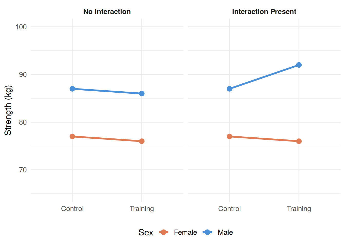
The clearest way to detect and communicate an interaction is through an interaction plot: a graph with the levels of one factor on the x-axis, the outcome variable on the y-axis, and separate lines for each level of the second factor. When the lines are parallel (or nearly so), there is no interaction. When the lines diverge, converge, or cross, an interaction is present. Figure 16.1 illustrates both patterns using simulated data.
Code
library(ggplot2)library(dplyr)set.seed(42)# Combine both scenarios into a single data frame for facetingd_schematic <-data.frame(Scenario =rep(c("No Interaction", "Interaction Present"), each =4),Group =rep(rep(c("Control", "Training"), each =2), 2),Sex =rep(rep(c("Female", "Male"), 2), 2),Mean =c(77, 87, 76, 86, # no interaction: parallel lines77, 87, 76, 92) # interaction: lines diverge for Male)d_schematic$Scenario <-factor(d_schematic$Scenario,levels =c("No Interaction", "Interaction Present"))d_schematic$Group <-factor(d_schematic$Group, levels =c("Control", "Training"))ggplot(d_schematic, aes(x = Group, y = Mean, group = Sex, color = Sex)) +geom_line(linewidth =1.2) +geom_point(size =3) +scale_color_manual(values =c("Female"="#E07B54", "Male"="#4A90D9"),name ="Sex") +facet_wrap(~ Scenario) +coord_cartesian(ylim =c(65, 100)) +labs(x =NULL, y ="Strength (kg)") +theme_minimal(base_size =13) +theme(legend.position ="bottom",strip.text =element_text(face ="bold"))
Figure 16.1: Schematic interaction plots. No Interaction (left): Parallel lines indicate that the Group effect is the same for both sexes. Interaction Present (right): Non-parallel lines indicate that the Group effect is larger for male than female participants.
ImportantAlways interpret the interaction before the main effects
When a factorial ANOVA yields a significant interaction, the main effects lose their simple interpretation. A main effect of Group that averages across two very different sex-specific patterns is technically accurate but substantively misleading. The cardinal rule is: check the interaction first. If it is significant, decompose it with simple effects analysis; do not interpret the main effects as stand-alone conclusions.
16.6 Between-subjects factorial ANOVA
16.6.1 Design and variance partitioning
In a two-way between-subjects ANOVA, every participant belongs to exactly one cell — one unique combination of Factor A and Factor B. The total variance in the outcome is partitioned into five sources: the main effect of A, the main effect of B, the A × B interaction, and the within-cell error. The F-ratio for each effect uses this same error term — the variance within cells — as the denominator.
The partitioning follows directly from the one-way ANOVA framework of Chapter 14, extended to two factors:
All three effects are tested against the same error term. The degrees of freedom follow from the number of levels: \(df_A = a - 1\) for a factor with \(a\) levels, \(df_{A \times B} = (a-1)(b-1)\) for the interaction, and \(df_{\text{error}} = N - ab\) where \(N\) is total sample size and \(ab\) is the number of cells[1].
In practice, you will never partition these sums of squares by hand. SPSS calculates them automatically. See the SPSS Tutorial: Factorial ANOVA for the full step-by-step procedure.
16.6.2 Worked example: Sex × Group on post-test strength
Research question: Did a 12-week training program improve strength at post-test, and did this effect differ between male and female participants?
Design: 2(Sex: Female, Male) × 2(Group: Control, Training) between-subjects ANOVA, outcome variable strength_kg at the post-test time point, \(N = 60\) (21 Female-Control, 12 Female-Training, 9 Male-Control, 18 Male-Training).
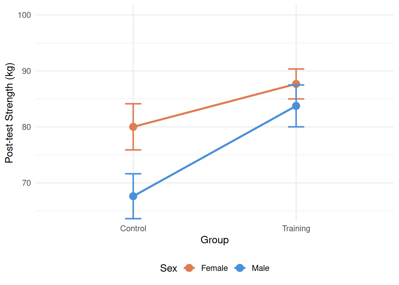
Interpretation: The interaction was not significant, F(1, 56) = 0.56, p = .457, η²_p = .010, indicating that the effect of training on post-test strength did not differ between male and female participants. Because the interaction was not significant, the main effects can be interpreted directly. The main effect of Group was significant, F(1, 56) = 5.22, p = .026, η²_p = .085, with the training group (M = 85.06 kg) outperforming the control group (M = 77.14 kg) at post-test regardless of sex — a moderate-sized between-groups difference. The main effect of Sex was not significant, F(1, 56) = 0.00, p = .974, η²_p = .000, confirming that male and female participants were similar in post-test strength when groups were collapsed.
Code
library(ggplot2)library(dplyr)set.seed(42)# Simulated data matching core_session.csv post-test valuesn_fc <-21; n_ft <-12; n_mc <-9; n_mt <-18df_between <-data.frame(sex =c(rep("Female",n_fc+n_ft), rep("Male",n_mc+n_mt)),group =c(rep("Control",n_fc), rep("Training",n_ft),rep("Control",n_mc), rep("Training",n_mt)),strength =c(rnorm(n_fc, 77.54, 14.70),rnorm(n_ft, 87.18, 8.21),rnorm(n_mc, 76.22, 12.92),rnorm(n_mt, 83.64, 14.72) ))summary_df <- df_between %>%group_by(sex, group) %>%summarise(M =mean(strength), SE =sd(strength)/sqrt(n()), .groups ="drop")ggplot(summary_df, aes(x = group, y = M, group = sex, color = sex)) +geom_line(linewidth =1.2) +geom_point(size =4) +geom_errorbar(aes(ymin = M - SE, ymax = M + SE), width =0.10, linewidth =0.9) +scale_color_manual(values =c("Female"="#E07B54", "Male"="#4A90D9"),name ="Sex") +scale_x_discrete(labels =c("Control", "Training")) +labs(x ="Group", y ="Post-test Strength (kg)") +coord_cartesian(ylim =c(65, 100)) +theme_minimal(base_size =13) +theme(legend.position ="bottom")
Figure 16.2: Post-test strength (kg) by Sex and Training Group. Error bars represent ± 1 standard error. Parallel lines confirm the absence of a statistically significant interaction: both male and female participants show similar training benefits.
NoteReal example: Equal training benefits across sex
The non-significant interaction in this example (η²_p = .010) tells a practically important story: the resistance training program produced equivalent relative gains in male and female participants. A physical therapist or strength coach can interpret this as evidence that the same training prescription was equally effective for both groups, without the need for sex-specific program modifications. Null interaction results are not failures — they are substantive findings about the boundary conditions of an effect.
16.6.3 Post hoc tests in between-subjects designs
When a factor has only two levels (as in the Sex × Group example above), a significant main effect identifies which two means differ without the need for additional tests — the only comparison available is the one already tested. When a factor has three or more levels, post hoc tests (such as Bonferroni correction or Tukey’s HSD) are applied to the marginal means for that factor, just as in the one-way ANOVA (Chapter 14). When an interaction is significant, post hoc testing proceeds through simple effects analysis rather than testing marginal means, as described below[5].
16.7 Mixed factorial ANOVA
16.7.1 The mixed design in movement science
The most common factorial design in training, rehabilitation, and motor learning research is the mixed factorial ANOVA, also called a split-plot design. It combines at least one between-subjects factor (such as Group) with at least one within-subjects factor (such as Time). This design is ideally suited to longitudinal training studies, where different groups of participants are measured repeatedly over the course of an intervention.
The mixed factorial answers a question that neither the between-subjects ANOVA nor the repeated measures ANOVA can answer alone: do groups differ in their trajectory of change over time? A training group that starts at the same strength level as a control group but gains 6 kg by post-test while the control group gains less than 1 kg shows a Group × Time interaction. This interaction is the scientific heart of most intervention studies in movement science[1,3].
16.7.2 Variance partitioning in the mixed design
The partitioning of variance in a mixed ANOVA is more complex than in the between-subjects case because there are two distinct error terms: one for between-subjects effects, and one for within-subjects effects. Consider a 2(Group) × 3(Time) design with \(n\) participants per group:
\(SS_{\text{Group}}\) captures variance among group means; \(SS_{\text{Subjects/Group}}\) — subjects nested within groups — is the error term for the Group F-ratio.
\(SS_{\text{Time}}\) captures variance among time-point means; \(SS_{\text{Group} \times \text{Time}}\) captures the interaction; and \(SS_{\text{Time} \times \text{Subjects/Group}}\) — the time-by-subjects-within-groups term — is the error for both the Time and the interaction F-ratios.
This produces three F-ratios with different denominators:
The between-subjects error (\(MS_{\text{Subjects/Group}}\)) is typically large — it reflects all the stable individual differences that make people different from one another in overall strength level. The within-subjects error (\(MS_{\text{Time} \times \text{Subjects/Group}}\)) is usually much smaller — it captures only how inconsistently each participant responds to time, stripped of individual baselines. This asymmetry is why the Time and interaction effects tend to have much higher statistical power than the Group (between-subjects) effect[1,6].
WarningCommon mistake: Using the wrong error term
Because the mixed ANOVA uses two different error terms, there is an important conceptual trap: the between-subjects F and the within-subjects F are not directly comparable in magnitude, even if they test effects of similar practical importance. A Group F of 2.5 and a Time F of 108 do not mean that Time is 43 times more important — they are evaluated against completely different sources of variance. Always focus on effect size (η²_p or ω²_p) to compare the practical magnitude of effects across different sources in a mixed ANOVA.
16.7.3 Sphericity in the mixed ANOVA
As introduced in Chapter 15, the sphericity assumption requires that the variances of all pairwise differences among the within-subjects factor levels be approximately equal. In a mixed ANOVA, this assumption applies to the within-subjects factor (Time) and the interaction term — both use the same within-subjects error. Mauchly’s test of sphericity should be inspected before reading the Time and interaction F-ratios. If the test is significant (suggesting sphericity is violated), apply the Greenhouse-Geisser correction when \(\hat{\varepsilon} < .75\) and the Huynh-Feldt correction when \(\hat{\varepsilon} \geq .75\)[6–8]. SPSS reports both corrections automatically.
16.7.4 Worked example: Group × Time on strength
Research question: Did strength change over a 12-week training program, and did the trajectory of change differ between the training and control groups?
Design: 2(Group: Control, Training) × 3(Time: Pre, Mid, Post) mixed ANOVA, Group = between-subjects factor, Time = within-subjects factor, \(n = 30\) per group, outcome variable strength_kg.
Table 16.3: Cell means and standard deviations (in parentheses) for strength (kg) by Group and Time.
Group
Pre
Mid
Post
Control
76.34 (13.70)
76.85 (13.87)
77.14 (13.98)
Training
79.67 (12.26)
81.69 (12.26)
85.06 (12.48)
Sphericity: For this dataset, Mauchly’s test of sphericity was not significant (a finding consistent with the very gradual and nearly uniform spread of difference variances across the three time points), so the sphericity-assumed F values are reported below.
Interpretation: The Group × Time interaction was highly significant, F(2, 116) = 61.00, p < .001, η²_p = .513, ω²_p = .400 — a large effect by any standard[9,10]. Because the interaction is significant, the main effects of Group and Time are interpreted cautiously and in the context of the interaction pattern. The main effect of Time was also significant, F(2, 116) = 108.55, p < .001, η²_p = .652, indicating that strength changed across time when both groups are averaged together. The main effect of Group was not significant, F(1, 58) = 2.52, p = .117, η²_p = .042 — but this is expected when the interaction is present: the groups start at similar levels and diverge over time, so their overall (time-averaged) means are not dramatically different.
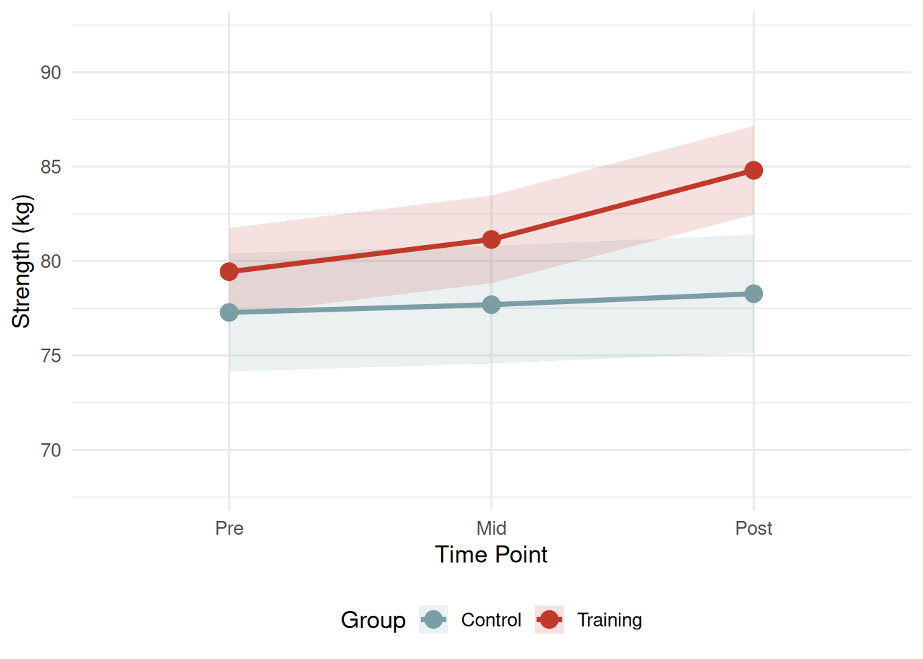
Figure 16.3 shows the interaction pattern clearly: the training group shows a progressive linear increase in strength from pre (M = 79.67 kg) to mid (M = 81.69 kg) to post (M = 85.06 kg), while the control group remains essentially flat across all three time points (76.34, 76.85, 77.14 kg). The lines diverge rather than cross, indicating a quantitative interaction: training benefits are not reversed in the control group, but they are substantially larger.
Code
library(ggplot2)library(dplyr)set.seed(42)n <-30id <-1:n# Simulate correlated within-subject data matching real means/SDspre_ctrl <-rnorm(n, 76.34, 13.70)mid_ctrl <- pre_ctrl +rnorm(n, 0.51, 0.80)post_ctrl <- pre_ctrl +rnorm(n, 0.80, 1.00)pre_train <-rnorm(n, 79.67, 12.26)mid_train <- pre_train +rnorm(n, 2.02, 1.20)post_train <- pre_train +rnorm(n, 5.39, 1.40)df_long <-data.frame(id =rep(1:(2*n), each =3),group =rep(c(rep("Control",n), rep("Training",n)), each =3),time =rep(c("Pre","Mid","Post"), 2*n),strength =c(rbind(pre_ctrl, mid_ctrl, post_ctrl),rbind(pre_train, mid_train, post_train)))df_long$time <-factor(df_long$time, levels =c("Pre","Mid","Post"))summary_df <- df_long %>%group_by(group, time) %>%summarise(M =mean(strength),SE =sd(strength)/sqrt(n()),.groups ="drop")ggplot(summary_df, aes(x = time, y = M, group = group,color = group, fill = group)) +geom_ribbon(aes(ymin = M - SE, ymax = M + SE), alpha =0.15, color =NA) +geom_line(linewidth =1.3) +geom_point(size =4) +scale_color_manual(values =c("Control"="#7B9EA6", "Training"="#C0392B"),name ="Group") +scale_fill_manual(values =c("Control"="#7B9EA6", "Training"="#C0392B"),name ="Group") +labs(x ="Time Point", y ="Strength (kg)") +coord_cartesian(ylim =c(68, 92)) +theme_minimal(base_size =13) +theme(legend.position ="bottom")
Figure 16.3: Strength (kg) across time by training group. Error bars represent ± 1 standard error of the mean. The diverging trajectories constitute the significant Group × Time interaction: the training group shows progressive strength gains while the control group remains essentially unchanged.
16.8 Simple effects analysis
16.8.1 What are simple effects?
When an interaction is statistically significant, the main effects provide an incomplete — and sometimes misleading — summary. The solution is simple effects analysis: testing the effect of one factor separately at each level of the other factor. In the Group × Time example, simple effects analysis asks two complementary questions:
Does strength change across Time within the Control group? (simple effect of Time at Control)
Does strength change across Time within the Training group? (simple effect of Time at Training)
Alternatively, the analysis can be “flipped” to ask about Group differences at each time point separately:
Do the groups differ at Pre? At Mid? At Post?
Both perspectives are valid; the choice depends on the research question. In training studies, the most theoretically interesting question is usually whether the intervention group changed — which motivates examining the simple effect of Time within each group. In cross-sectional comparisons, examining Group differences at each time point may be more informative.
16.8.2 Interpreting simple effects in the Group × Time example
Examining Table 16.3 and Figure 16.3, the simple effects pattern is apparent. Within the Control group, the three time-point means (76.34, 76.85, 77.14 kg) differ by less than 1 kg across the entire 12-week period — a negligible and statistically non-significant change. Within the Training group, strength increased by 2.02 kg from Pre to Mid, and by an additional 3.37 kg from Mid to Post, for a total gain of 5.39 kg — a large and highly significant change that mirrors the repeated measures ANOVA findings from Chapter 15.
When examining Group differences at each time point, the groups start comparably at Pre (76.34 vs. 79.67 kg, difference = 3.33 kg, non-significant) but diverge progressively at Mid (76.85 vs. 81.69, difference = 4.84 kg) and Post (77.14 vs. 85.06 kg, difference = 7.92 kg, statistically significant). This divergence pattern is the visual signature of a significant interaction and the most compelling evidence that the training program produced meaningful physiological adaptation.
In SPSS, simple effects are accessed through the General Linear Model → Repeated Measures dialog by clicking Options → Compare main effects for within-subjects factors, or by running separate one-way ANOVAs after splitting the file by one factor. See the SPSS Tutorial: Factorial ANOVA for step-by-step instructions.
TipUse interaction plots before running simple effects
Before running formal simple effects tests, always examine the interaction plot. The plot tells you where the interaction is — which group diverges, and at which time point. Running simple effects blindly, without looking at the plot, can lead to testing combinations that are not theoretically interesting and interpreting numerically significant but practically trivial differences.
16.9 Within-within factorial ANOVA
A within-within (or fully within-subjects) factorial design measures all participants under every combination of both factors. In movement science, this might arise when participants complete tasks under multiple difficulty levels (Factor A: easy, medium, hard) on multiple occasions (Factor B: Day 1, Day 7, Day 14). Each participant contributes a data point to every one of the \(a \times b\) cells.
The appeal is statistical power: because individual differences are removed for every source of variance, both main effects and the interaction benefit from the within-subject error terms. The limitation is practical feasibility — participants must complete all condition combinations, raising concerns about fatigue, learning, and carryover effects that can corrupt the independence assumption. Counterbalancing (randomizing the order of conditions) is essential in within-within designs[1].
Variance partitioning in the within-within design produces separate within-subject error terms for each source of variance: \(SS_{\text{A} \times \text{Subjects}}\) for Factor A, \(SS_{\text{B} \times \text{Subjects}}\) for Factor B, and \(SS_{\text{A} \times \text{B} \times \text{Subjects}}\) for the interaction. The sphericity assumption must be evaluated for every within-subjects factor with three or more levels, and corrections applied as needed. Because of this complexity, SPSS’s General Linear Model → Repeated Measures module handles within-within designs using the same interface as the one-way repeated measures ANOVA from Chapter 15 — simply define both within-subjects factors when setting up the model.
16.10 Effect sizes for factorial designs
16.10.1 Partial eta-squared and partial omega-squared
As in the one-way ANOVA (Chapter 14) and repeated measures ANOVA (Chapter 15), the recommended effect size measures for factorial designs are partial eta-squared (η²_p) and the less-biased partial omega-squared (ω²_p). The partial qualifier is critical: each effect’s η²_p is computed using only that effect’s SS and the error SS, ignoring the SS from other effects. This makes partial η²_p appropriately reflect each effect’s size holding other effects constant, rather than as a proportion of total variance[10].
For a mixed ANOVA, the “error” in the formula differs by effect type: the between-subjects error (\(SS_{\text{Subjects/Group}}\)) is used for the Group main effect, while the within-subjects error (\(SS_{\text{Time} \times \text{Subjects/Group}}\)) is used for the Time main effect and the interaction.
Partial omega-squared corrects for positive bias by adjusting both the numerator and denominator:
where \(p\) is the number of within-subjects levels (for within-subject terms) or 1 (for between-subjects terms), and \(N\) is the total number of participants[10].
Common benchmarks for partial η²_p from[9]: small ≈ .01, medium ≈ .06, large ≥ .14. These benchmarks apply cautiously in movement science contexts, where large effects (η²_p > .50) are common in well-controlled laboratory training studies with physiological outcome variables, but rare in field studies with noisy measurement.
16.10.2 Cohen’s f for power calculations
For factorial ANOVA power planning in G*Power, the required effect size metric is Cohen’s f rather than η²_p. The conversion is:
\[f = \sqrt{\frac{\eta^2_p}{1 - \eta^2_p}}\]
For the Group × Time interaction (η²_p = .513): \(f = \sqrt{.513 / .487} = \sqrt{1.053} = 1.03\) — a very large effect. For the between-subjects Group effect (η²_p = .042): \(f = \sqrt{.042 / .958} = 0.21\) — a small-to-medium effect. These values reflect the fundamental asymmetry of the mixed design: within-subject effects enjoy far better statistical power than between-subject effects, because the former are tested against a much smaller error term.
16.11 Sample size and power for factorial designs
Power planning for factorial ANOVAs in GPower follows the same logic as for one-way ANOVA (Chapter 14), using the F-test: ANOVA: Fixed effects, special, main effects, and interactions* option. The key inputs for each effect are: the effect size f, the desired power (typically .80 or .90), the alpha level (.05), the numerator degrees of freedom for the effect being planned, and the total sample size.
For a mixed ANOVA, power calculations for the Group main effect and for the Group × Time interaction require different approaches because they use different error terms. GPower’s ANOVA: Repeated Measures, between-within interaction* option handles this automatically and is the recommended starting point for planning mixed factorial studies. The critical additional input is the correlation among repeated measures — the expected correlation between time-point scores within the same participant. As discussed in Chapter 15, higher within-subject correlation increases the power of within-subjects tests by reducing the within-subjects error. In training studies using the core_session.csv dataset, the pre-mid-post correlations in strength are approximately r = .96 to .98, explaining the extremely high power of the Time and interaction effects in this example.
TipG*Power and SPSS for factorial power planning
For between-subjects factorial designs, use GPower → F-test: ANOVA: Fixed effects, omnibus, one-way* (treating each effect as a planned comparison) or the special main effects option. For mixed designs, use GPower → F-test: ANOVA: Repeated Measures, between-within interaction. SPSS 31 and later include a built-in power analysis module (Analyze → Power Analysis → One-way ANOVA* or General Linear Model) that can estimate power for each effect in a factorial design directly from pilot data. The Statistical Calculators appendix also includes an interactive power tool for exploration.
16.12 Reporting factorial ANOVA in APA style
16.12.1 Template
A two-way between-subjects ANOVA revealed no significant interaction between [Factor A] and [Factor B], F(df1, df2) = [value], p = [value], η²_p = [value], suggesting that the effect of [Factor B] did not differ by [Factor A]. There was a significant main effect of [Factor B], F(df1, df2) = [value], p = [value], η²_p = [value], ω²_p = [value], with the [level] group (M = [value], SD = [value]) scoring higher than the [level] group (M = [value], SD = [value]).
For a mixed ANOVA with a significant interaction:
A 2(Group) × 3(Time) mixed ANOVA revealed a significant Group × Time interaction, F(2, 116) = 61.00, p < .001, η²_p = .51, ω²_p = .40. Simple effects analysis indicated that strength increased significantly across time in the training group ([pre → post reporting here]) but not in the control group. The main effect of Time was significant, F(2, 116) = 108.55, p < .001, η²_p = .65, and the main effect of Group was not significant, F(1, 58) = 2.52, p = .117, η²_p = .04.
16.12.2 Full APA example: Group × Time mixed ANOVA
A 2 (Group: control, training) × 3 (Time: pre, mid, post) mixed ANOVA was conducted with strength_kg as the dependent variable. Mauchly’s test of sphericity indicated that the sphericity assumption was not violated, W = .93, p = .059. The Group × Time interaction was statistically significant, F(2, 116) = 61.00, p < .001, η²_p = .51, ω²_p = .40, indicating that the two groups followed different strength trajectories across the 12-week program. Simple effects analysis revealed a significant effect of Time within the training group, with progressive gains from pre-test (M = 79.67 kg, SD = 12.26) to mid-test (M = 81.69 kg, SD = 12.26) and post-test (M = 85.06 kg, SD = 12.48), consistent with the repeated measures analysis reported in Chapter 15. The effect of Time was not significant within the control group, which remained essentially unchanged across the three assessments (76.34, 76.85, 77.14 kg). The main effect of Time was significant, F(2, 116) = 108.55, p < .001, η²_p = .65, and the main effect of Group was not significant, F(1, 58) = 2.52, p = .117, η²_p = .04.
16.13 Common pitfalls and best practices
16.13.1 Pitfall 1: Interpreting main effects when the interaction is significant
Perhaps the most frequent mistake in factorial ANOVA reporting is stating a significant main effect without acknowledging — or even examining — the interaction. If a 2 × 2 ANOVA yields significant main effects of both Sex and Group but also a significant Sex × Group interaction, the “main effect of Group” averaged across both sexes is a statistical fiction: it accurately describes neither the male pattern nor the female pattern, but only an average of two different patterns. Always test the interaction first, and if it is significant, decompose it before making any statements about main effects.
16.13.2 Pitfall 2: Confusing “no significant interaction” with “no interaction”
When Mauchly’s test or the interaction F-ratio is non-significant, students sometimes conclude that “there is no interaction” and proceed as though the parallel-lines assumption is perfectly supported. The correct statement is that the data are consistent with the absence of an interaction — but a study with low power cannot distinguish a small interaction from no interaction. Report the η²_p for the interaction even when p > .05, and note whether the study was adequately powered to detect a small interaction[11].
16.13.3 Pitfall 3: Using the wrong error term in a mixed ANOVA
The between-subjects Group effect and the within-subjects Time effect in a mixed ANOVA are tested against different error terms. If you compute F values manually (or modify syntax in SPSS), using the within-subjects error for the Group effect will produce an artificially large F, because \(MS_{\text{within error}}\) is much smaller than \(MS_{\text{Subjects/Group}}\). SPSS handles this automatically in the Repeated Measures GLM — but understanding which error term each F uses is essential for interpreting the output correctly.
16.13.4 Pitfall 4: Failing to report effect sizes for all effects
Journals in movement science and kinesiology increasingly require effect size reporting for every source of variance, not just the primary outcome. Report η²_p (and ideally ω²_p) for the main effect of Group, the main effect of Time, and the interaction. Readers need all three to evaluate whether a non-significant Group effect, for example, was simply underpowered or was genuinely trivial[12].
16.14 Chapter summary
Factorial ANOVA extends the one-way framework to situations where two or more independent variables operate simultaneously on a single outcome. The central conceptual contribution of the factorial design is the interaction effect: evidence that the influence of one factor depends on the level of another. Interactions are among the most important and scientifically interesting findings in movement science research, and detecting them requires simultaneous manipulation or observation of multiple factors — something that a series of one-way ANOVAs cannot accomplish.
The between-subjects factorial ANOVA is appropriate when participants are randomly assigned to or naturally classified into cells defined by unique combinations of factor levels, and every cell is tested against a single pooled error term. The mixed factorial ANOVA is the workhorse of longitudinal intervention research: it separates the large variability among individuals (the between-subjects error) from the much smaller variability in how participants change over time (the within-subjects error), yielding powerful tests of training trajectories and Group × Time interactions. The worked example in this chapter — training group versus control across three time points on strength_kg — produced a Group × Time interaction of η²_p = .51, demonstrating that the training program not only improved strength but did so with a trajectory that was fundamentally different from the control group’s stable baseline[1,10].
Effect size reporting using η²_p and ω²_p is essential for every factorial source, and partial effect sizes are the appropriate choice because they express each effect’s magnitude relative to its own error term. Power planning, whether through G*Power or SPSS’s built-in module, must account for the asymmetry between between-subjects and within-subjects tests: the interaction in a mixed design is typically much better powered than the between-subjects main effect, and sample size decisions must reflect which effect is the primary focus of inference. Chapter 17 extends the analysis of covariance framework, adding a continuous covariate to the between-groups model to improve precision and control for baseline differences — a natural complement to the designs developed here.
Running two separate one-way ANOVAs tests each factor in isolation and cannot detect whether the effect of one factor depends on the level of another — the interaction. Factorial ANOVA simultaneously estimates main effects and the interaction while using a single model, keeping the familywise error rate under control. Additionally, the factorial approach often uses a smaller error term than separate one-way tests, because variance attributable to all factors is removed before estimating error, yielding more powerful tests. The interaction is the exclusive contribution of the factorial design — it simply does not exist in a series of separate analyses.
In a mixed factorial ANOVA, Group (a between-subjects factor) and Time (a within-subjects factor) are evaluated against different error terms. The Group F uses the between-subjects error — the variance among individual participant means, which includes all stable individual differences in strength. This is a large and noisy error term. The Time F uses the within-subjects error — the variance in how individuals change across time points relative to their own trajectories — which is far smaller. Because the same MS_effect is divided by a much smaller denominator, within-subjects F-ratios are typically larger than between-subjects F-ratios even when the underlying effect sizes are comparable. Always compare effects using η²_p or ω²_p, not F values, when they come from different error terms.
Not wrong — technically accurate, but substantively incomplete. The main effect of Group in this analysis (p = .117) averages across all three time points. Because the training and control groups start at similar strength levels and only diverge over time, their time-averaged means are not dramatically different, yielding a non-significant omnibus Group comparison. The interaction reveals the more informative pattern: the change trajectories diverge significantly. In factorial designs with significant interactions, main effects describe a simplified picture that may be misleading without the interaction context. The recommended practice is to interpret the interaction first, then report the main effects with explicit acknowledgment that they must be understood in light of the interaction.
The conventional choice is to place the factor with more levels on the x-axis and use separate lines for the factor with fewer levels — this maximizes the visual resolution of the interaction pattern. In a Group × Time design with 2 groups and 3 time points, placing Time on the x-axis and drawing separate lines for Control and Training produces a clear picture of how trajectories diverge over time. If both factors have the same number of levels, the theoretically primary factor (the one whose moderation is of greatest interest) typically goes on the x-axis. The goal of the interaction plot is to make the presence or absence of an interaction maximally visible, so any arrangement that clearly shows whether the lines are parallel or diverging is defensible.
Several elements are missing for a complete factorial ANOVA report. First, the interaction test result and its effect size should be reported before interpreting the main effect — η²_p = .085 for Group is only interpretable if the interaction is non-significant. Second, the main effect of Sex (the other factor) should be reported. Third, descriptive statistics — means and standard deviations for each group — should accompany the omnibus F-test. Fourth, partial omega-squared (ω²_p) provides a less biased effect size estimate and should ideally accompany η²_p. A complete report would state: “The Sex × Group interaction was not significant, F(1, 56) = 0.56, p = .457, η²_p = .010. The main effect of Group was significant, F(1, 56) = 5.22, p = .026, η²_p = .085, ω²_p = .069, with the training group (M = 85.06 kg, SD = 12.48) exceeding the control group (M = 77.14 kg, SD = 13.98).”
No — this approach is problematic on two counts. First, it creates an inflated familywise Type I error rate: six tests at α = .05 raises the probability of at least one false positive to approximately 26%. Second, if sex is not one of the factors in the model, comparing training and control groups separately by sex adds a variable that was never modeled, making the results uninterpretable in the context of the original ANOVA. The appropriate procedure is simple effects analysis within the ANOVA framework: test the effect of Group at each level of Time (or vice versa) using the same error term as the original model, with Bonferroni correction applied across the simple effects comparisons. This keeps Type I error controlled and ensures interpretive consistency with the omnibus test.
NoteRead further
For an authoritative treatment of factorial ANOVA in experimental research, including extended coverage of mixed designs and power planning, see[1].[2] provides a software-focused introduction with detailed SPSS and R walkthroughs. For effect size reporting guidance specific to repeated-measures and factorial designs,[10] is the primary methodological reference, and[9] remains the foundational source on statistical power and the f metric.
NoteNext chapter
Chapter 17 introduces Analysis of Covariance (ANCOVA), which adds a continuous covariate to the ANOVA framework to statistically control for pre-existing differences among groups. ANCOVA is especially valuable in pre-test/post-test designs where randomization does not perfectly equate groups at baseline — a common situation in applied exercise science and rehabilitation research.
1. Maxwell, S. E., Delaney, H. D., & Kelley, K. (2018). Designing experiments and analyzing data: A model comparison perspective (3rd ed.). Routledge.
2. Field, A. (2018). Discovering statistics using IBM SPSS statistics (5th ed.). SAGE Publications.
4. Vincent, W. J. (2005). Statistics in kinesiology.
5. Tukey, J. W. (1949). Comparing individual means in the analysis of variance. Biometrics, 5(2), 99–114. https://doi.org/10.2307/3001913
6. Girden, E. R. (1992). ANOVA: Repeated measures. Sage.
7. Greenhouse, S. W., & Geisser, S. (1959). On methods in the analysis of profile data. Psychometrika, 24(2), 95–112. https://doi.org/10.1007/BF02289823
8. Huynh, H., & Feldt, L. S. (1976). Estimation of the box correction for degrees of freedom from sample data in randomized block and split-plot designs. Journal of Educational Statistics, 1(1), 69–82. https://doi.org/10.3102/10769986001001069
9. Cohen, J. (1988). Statistical power analysis for the behavioral sciences (2nd ed.). Lawrence Erlbaum Associates.
10. Olejnik, S., & Algina, J. (2003). Generalized eta and omega squared statistics: Measures of effect size for some common research designs. Psychological Methods, 8(4), 434–447. https://doi.org/10.1037/1082-989X.8.4.434
11. Button, K. S., Ioannidis, J. P. A., Mokrysz, C., Nosek, B. A., Flint, J., Robinson, E. S. J., & Munafò, M. R. (2013). Power failure: Why small sample size undermines the reliability of neuroscience. Nature Reviews Neuroscience, 14, 365–376. https://doi.org/10.1038/nrn3475
12. Lakens, D. (2013). Calculating and reporting effect sizes to facilitate cumulative science: A practical primer for t-tests and ANOVAs. Frontiers in Psychology, 4, 863. https://doi.org/10.3389/fpsyg.2013.00863