Appendix K — Calculating Measures of Central Tendency in SPSS
Mean, Median, and Mode Using SPSS 31
K.1 Purpose & Outcomes
This tutorial teaches you how to calculate and interpret measures of central tendency using SPSS 31. By the end, you will be able to compute the mean, median, and mode for continuous and categorical variables using both the Frequencies and Descriptives procedures. You will learn when to use each procedure, how to interpret the output tables, and how to report these statistics in APA format. Additionally, you will understand which measure of central tendency is most appropriate for different types of data and distributions.
K.2 Why This Matters
Measures of central tendency are fundamental descriptive statistics that summarize the typical or central value in a dataset. Understanding how to calculate and interpret the mean, median, and mode is essential for describing your data, identifying patterns, and making informed decisions about which statistical tests to use. These statistics form the foundation for more advanced analyses and are required components of nearly every research report and data analysis project.
K.3 Understanding Measures of Central Tendency
Before diving into SPSS procedures, it’s important to understand what each measure represents and when to use it.
K.3.1 The Mean
The mean (arithmetic average) is calculated by summing all values and dividing by the number of observations. It’s the most commonly used measure of central tendency for continuous data. The mean is sensitive to extreme values (outliers), which can pull it away from the center of the distribution. Use the mean when your data is approximately normally distributed and measured on an interval or ratio scale.
Formula: \(\bar{X} = \frac{\sum X}{N}\)
K.3.2 The Median
The median is the middle value when data is arranged in order. Half of the values fall above the median and half fall below it. The median is resistant to outliers and extreme values, making it a better choice than the mean for skewed distributions. Use the median for ordinal data or when your continuous data contains outliers or is substantially skewed.
K.3.3 The Mode
The mode is the most frequently occurring value in a dataset. A distribution can have one mode (unimodal), two modes (bimodal), or more (multimodal). The mode is the only measure of central tendency appropriate for nominal (categorical) data, though it can be calculated for any type of data. For continuous variables with many unique values, the mode may not be particularly informative.
K.4 Two SPSS Procedures for Central Tendency
SPSS offers two main procedures for calculating measures of central tendency: Frequencies and Descriptives. Understanding when to use each is important for efficient data analysis.
K.4.1 When to Use Frequencies
Use the Frequencies procedure when you want:
- All three measures of central tendency (mean, median, and mode)
- Frequency tables showing how often each value occurs
- Charts and graphs (histograms, bar charts)
- Analysis of categorical or ordinal variables
- Percentiles and quartiles
The Frequencies procedure is more comprehensive but produces more output, which can be overwhelming for datasets with many unique values.
K.4.2 When to Use Descriptives
Use the Descriptives procedure when you want:
- Quick summary statistics for continuous variables
- The mean and standard deviation (but not median or mode)
- Compact output without frequency tables
- To analyze multiple variables efficiently
- Standardized (z-score) values
The Descriptives procedure is streamlined and efficient for continuous data but does not provide the median or mode.
K.5 Method 1: Using Frequencies
The Frequencies procedure provides the most comprehensive output for calculating measures of central tendency, including all three statistics plus frequency distributions.
K.5.1 Step-by-Step Instructions
Step 1: Open Your Dataset
Before beginning, ensure your data file is open in SPSS. If you need to open a file, go to File > Open > Data and navigate to your .sav file.
Step 2: Access the Frequencies Dialog
Navigate to the menu bar and select:
Analyze > Descriptive Statistics > Frequencies
This opens the Frequencies dialog box.
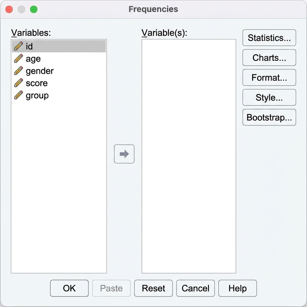
Step 3: Select Your Variable(s)
In the Frequencies dialog:
- On the left side, you’ll see a list of all variables in your dataset
- Click on the variable(s) you want to analyze (e.g.,
test_score,age,reaction_time) - Click the arrow button to move selected variables to the Variable(s): box on the right
- You can select multiple variables to analyze them all at once
By default, SPSS will display frequency tables showing every unique value and its count. For continuous variables with many unique values, these tables can be very long. If you only want the statistics (not the full frequency table), click the Format button and select “Suppress tables with more than N categories” or simply uncheck “Display frequency tables” at the bottom of the main dialog.
Step 4: Request Statistics
Click the Statistics button to open the Frequencies: Statistics subdialog.
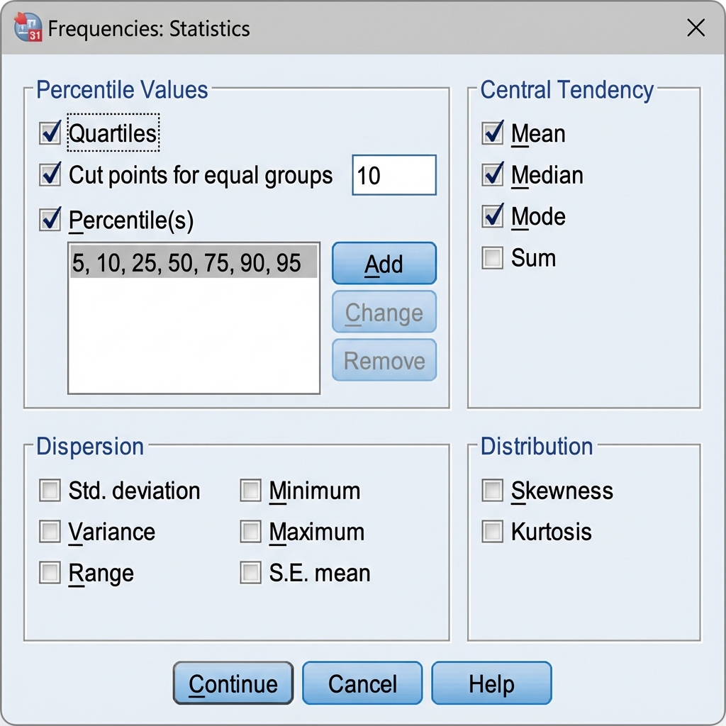
In the Central Tendency section, check the boxes for:
- ☑ Mean — arithmetic average
- ☑ Median — middle value
- ☑ Mode — most frequent value
You can also select additional statistics in other sections:
- Percentile Values: Quartiles, specific percentiles
- Dispersion: Standard deviation, variance, range
- Distribution: Skewness, kurtosis
Once you’ve made your selections, click Continue to return to the main dialog.
Step 5: Run the Analysis
Click OK to execute the analysis. SPSS will generate output in the Output Viewer window.
K.5.2 Interpreting Frequencies Output
The output will contain a Statistics table showing your requested measures of central tendency.

Reading the Output Table:
- N Valid: Number of cases with non-missing values
- N Missing: Number of cases with missing values
- Mean: The arithmetic average (e.g., 78.40)
- Median: The middle value (e.g., 80.00)
- Mode: The most frequent value (e.g., 85)
Interpretation Example:
For a test score variable with Mean = 78.40, Median = 80.00, and Mode = 85:
- The average test score is 78.40 points
- Half of students scored below 80 and half scored above 80
- The most common score was 85 (more students earned this score than any other)
- The mean is lower than the median, suggesting a slight negative skew (some low scores pulling the mean down)
K.5.3 Syntax for Frequencies
For reproducibility, you can use syntax to run the Frequencies procedure:
* Calculate measures of central tendency using Frequencies.
FREQUENCIES VARIABLES=test_score
  /STATISTICS=MEAN MEDIAN MODE
  /ORDER=ANALYSIS.
To suppress the frequency table and show only statistics:
* Calculate statistics without frequency table.
FREQUENCIES VARIABLES=test_score
  /STATISTICS=MEAN MEDIAN MODE
  /FORMAT=NOTABLE
  /ORDER=ANALYSIS.
K.6 Method 2: Using Descriptives
The Descriptives procedure is faster and more efficient for continuous variables when you only need the mean and don’t require the median or mode.
K.6.1 Step-by-Step Instructions
Step 1: Access the Descriptives Dialog
Navigate to the menu bar and select:
Analyze > Descriptive Statistics > Descriptives
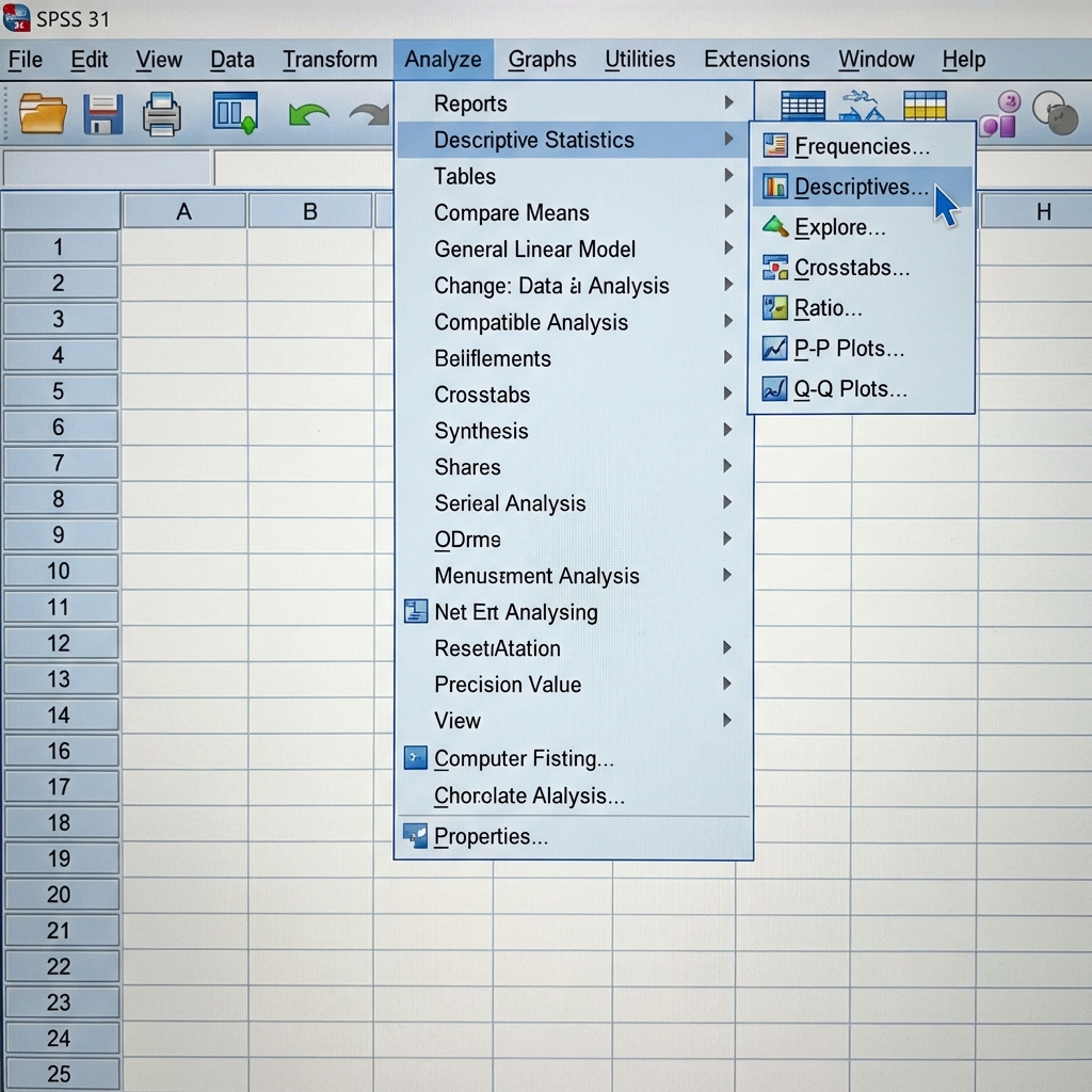
This opens the Descriptives dialog box.

Step 2: Select Your Variable(s)
- From the variable list on the left, select the variable(s) you want to analyze
- Click the arrow button to move them to the Variable(s): box
- You can analyze multiple variables simultaneously
Step 3: Configure Options
Click the Options button to specify which statistics to calculate.
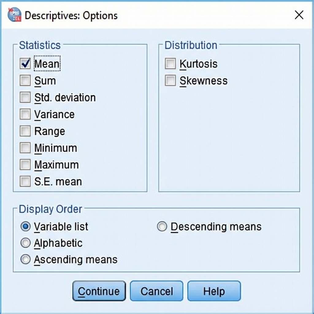
In the Options dialog:
Statistics Section:
- ☑ Mean — This is checked by default and is the primary measure from Descriptives
- You can also select: Sum, Std. deviation, Variance, Range, Minimum, Maximum, S.E. mean
Distribution Section:
- Kurtosis and Skewness (useful for assessing normality)
Display Order:
- Choose how variables are ordered in the output table
The Descriptives procedure does not calculate the median or mode. If you need these statistics, you must use the Frequencies procedure instead.
Click Continue to return to the main dialog, then click OK to run the analysis.
K.6.2 Interpreting Descriptives Output
The output displays a compact table with summary statistics for each variable.
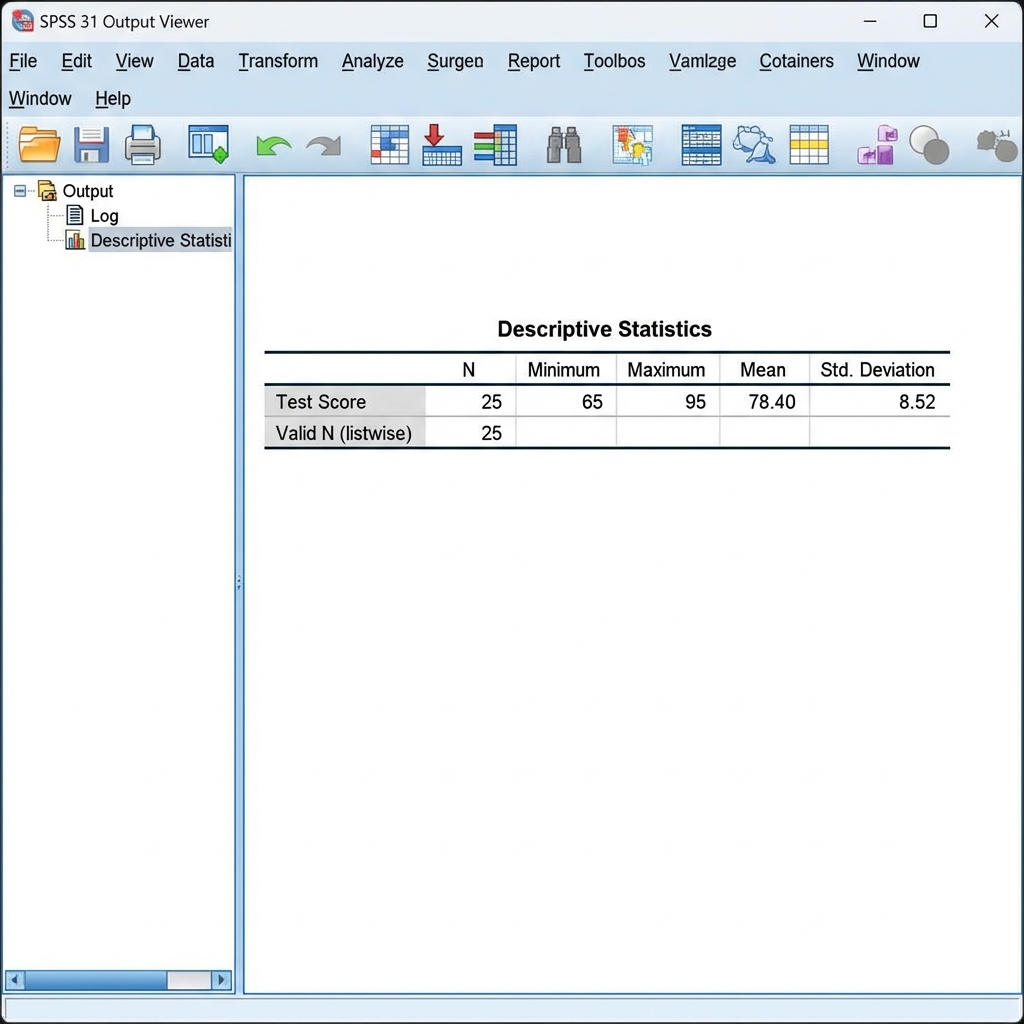
Reading the Output Table:
- N: Number of valid cases
- Minimum: Lowest value in the dataset
- Maximum: Highest value in the dataset
- Mean: Arithmetic average
- Std. Deviation: Measure of spread around the mean
Interpretation Example:
For a test score variable with N=25, Min=65, Max=95, Mean=78.40, SD=8.52:
- 25 students completed the test
- Scores ranged from 65 to 95 points
- The average score was 78.40 points
- Most scores fell within approximately 8.52 points of the mean
K.6.3 Syntax for Descriptives
* Calculate descriptive statistics including mean.
DESCRIPTIVES VARIABLES=test_score
  /STATISTICS=MEAN STDDEV MIN MAX.
K.7 Comparing the Two Procedures
| Feature | Frequencies | Descriptives |
|---|---|---|
| Mean | ✓ Yes | ✓ Yes |
| Median | ✓ Yes | ✗ No |
| Mode | ✓ Yes | ✗ No |
| Frequency Tables | ✓ Yes | ✗ No |
| Charts/Graphs | ✓ Yes | ✗ No |
| Compact Output | ✗ No | ✓ Yes |
| Best For | Categorical/Ordinal data, complete analysis | Continuous data, quick summaries |
| Z-scores | ✗ No | ✓ Yes (optional) |
K.8 Choosing the Right Measure
The choice of which measure of central tendency to use depends on your data type and distribution:
K.8.1 Use the Mean When:
- Data is measured on an interval or ratio scale
- Distribution is approximately symmetric (not heavily skewed)
- No extreme outliers are present
- You need to perform further calculations (e.g., t-tests, ANOVA)
K.8.2 Use the Median When:
- Data is ordinal (ranked)
- Distribution is skewed
- Outliers are present
- You want a measure resistant to extreme values
K.8.3 Use the Mode When:
- Data is nominal (categorical)
- You want to identify the most common category
- Data is bimodal or multimodal (multiple peaks)
For continuous data, report both the mean and median. If they differ substantially, this indicates skewness and you should investigate further. For example, income data is typically right-skewed, so the median provides a better representation of the “typical” income than the mean.
K.9 Reporting Results in APA Format
When reporting measures of central tendency in research papers or assignments, follow APA style guidelines:
K.9.1 Reporting the Mean
“The mean 20-m sprint time was 3.79 s (SD = 0.35, N = 60).”
or in a sentence:
“Participants completed the 20-m sprint in an average of 3.79 seconds (SD = 0.35).”
K.9.2 Reporting the Median
“The median sprint time was 3.80 s (IQR = 3.54–4.03 s).”
Note: IQR = Interquartile Range (25th to 75th percentile), which is the appropriate measure of spread for the median.
K.9.3 Reporting the Mode
“The modal response category was ‘Agree’ (n = 45, 45%).”
Note: The mode is most useful for categorical data. For continuous variables like sprint time, the mode may not be informative.
K.9.4 Reporting All Three
“Descriptive statistics for 20-m sprint time revealed a mean of 3.79 s (SD = 0.35), a median of 3.80 s, and a mode of 3.44 s. The similarity between the mean and median indicates an approximately symmetric distribution.”
K.9.5 In a Table
| Variable | N | M | Mdn | SD | Range |
|---|---|---|---|---|---|
| Sprint Time (s) | 60 | 3.79 | 3.80 | 0.35 | 2.90–4.45 |
| VO₂max (mL·kg⁻¹·min⁻¹) | 60 | 41.34 | 41.55 | 6.82 | 26.90–56.50 |
Note. M = mean; Mdn = median; SD = standard deviation. Pre-training time point (N = 60).
K.10 Sample Dataset for This Tutorial
We will use the Core Dataset from this book, specifically the core_session.csv file. This dataset comes from a mixed neuromuscular training study with recreationally active adults.
Click to download: core_session.csv
For complete information about this dataset, see the Core Dataset Overview and Core Dataset Codebook chapters.
K.10.1 Variables We’ll Analyze
For this tutorial, we’ll focus on these continuous variables:
- sprint_20m_s: 20-meter sprint time in seconds (lower is better)
- vo2_mlkgmin: Aerobic capacity estimate in mL·kg⁻¹·min⁻¹ (higher is better)
- age_years: Participant age in years
We’ll primarily use sprint_20m_s at the pre time point to demonstrate calculating measures of central tendency.
K.11 Practical Example: Complete Workflow
Let’s walk through a complete example using the 20-meter sprint times from the Core Dataset.
K.11.1 Scenario
You have collected 20-meter sprint times from participants at baseline (pre-intervention) and want to describe the central tendency of sprint performance in your sample.
K.11.2 Step 1: Import and Prepare the Data
- Download
core_session.csvfrom the link above - Open SPSS and import the file using File > Open > Data
- Save it as
core_session.savin your data folder
Since the dataset contains three time points (pre, mid, post), we need to filter to analyze only the baseline (pre) measurements.
Using Menus:
- Go to Data > Select Cases
- Choose “If condition is satisfied” and click If
- Enter:
time = "pre" - Click Continue, then OK
Using Syntax:
* Select only pre-intervention cases.
SELECT IF (time = "pre").
EXECUTE.
K.11.3 Step 2: Examine the Data
Look at the Data View to see the sprint times. Check for obvious errors or outliers. Sprint times should be in the range of approximately 2.5 to 5.0 seconds for recreationally active adults.
K.11.4 Step 3: Run Frequencies
Since you want all three measures of central tendency:
- Go to Analyze > Descriptive Statistics > Frequencies
- Move
sprint_20m_sto the Variable(s) box - Click Statistics and check Mean, Median, and Mode
- Also check Standard deviation and Range under Dispersion
- Click Continue, then OK
Syntax:
* Calculate measures of central tendency for sprint time.
FREQUENCIES VARIABLES=sprint_20m_s
  /STATISTICS=MEAN MEDIAN MODE STDDEV RANGE MIN MAX
  /FORMAT=NOTABLE
  /ORDER=ANALYSIS.
K.11.5 Step 4: Interpret the Output
Examine the Statistics table. For sprint_20m_s at pre-training (N = 60), you should see:
Statistics
                        sprint_20m_s
N        Valid           60
         Missing          0
Mean                     3.79
Median                   3.80
Mode                     3.44
Std. Deviation           .35
Minimum                  2.90
Maximum                  4.45
Range 1.55- N Valid = 60: All 60 pre-training participants have complete data
- Mean = 3.79 s: The average 20-m sprint time
- Median = 3.80 s: Half of participants were faster than 3.80 s, half were slower
- Mode = 3.44 s: The most common sprint time (for continuous data, mode is less informative)
- Std. Deviation = 0.35 s: Typical deviation from the mean
- Range = 1.55 s: Difference between fastest (2.90 s) and slowest (4.45 s)
K.11.6 Step 5: Assess the Distribution
Since the mean (3.79 s) is virtually identical to the median (3.80 s), the distribution appears approximately symmetric with no substantial skewness. This suggests the data is roughly normally distributed.
K.11.7 Step 6: Create a Visualization
To visualize the distribution:
- In the Frequencies dialog, click Charts
- Select Histograms and check “Show normal curve on histogram”
- Click Continue, then OK
Syntax:
* Create histogram with normal curve.
FREQUENCIES VARIABLES=sprint_20m_s
  /HISTOGRAM NORMAL
  /FORMAT=NOTABLE.
The histogram will show the shape of the distribution and help you identify any outliers or unusual patterns.
K.11.8 Step 7: Report the Results
“Twenty-meter sprint times at baseline (N = 60) ranged from 2.90 to 4.45 seconds, with a mean of 3.79 s (SD = 0.35) and a median of 3.80 s. The distribution was approximately symmetric, as evidenced by the close agreement between the mean and median, indicating that the mean provides an appropriate measure of central tendency for this variable.”
K.12 Common Pitfalls and Troubleshooting
K.12.1 Pitfall 1: Using the Mean for Skewed Data
Problem: Reporting only the mean when data is heavily skewed can be misleading.
Solution: Always check the distribution. If the mean and median differ substantially, report both and note the skewness. Consider using the median as the primary measure for skewed data.
K.12.2 Pitfall 2: Missing Values
Problem: SPSS excludes cases with missing values, which can affect your results.
Solution: Always check the “N Valid” and “N Missing” in your output. Investigate why data is missing and consider whether it’s missing at random or systematically.
K.12.3 Pitfall 3: Inappropriate Mode for Continuous Data
Problem: For continuous variables with many unique values, the mode may not be meaningful.
Solution: The mode is most useful for categorical data or discrete variables. For continuous data, focus on the mean and median.
K.12.4 Pitfall 4: Confusing Procedures
Problem: Using Descriptives when you need the median or mode.
Solution: Remember: Frequencies gives you all three measures; Descriptives only gives you the mean. Choose the procedure based on what statistics you need.
K.12.5 Pitfall 5: Not Checking for Outliers
Problem: Extreme values can dramatically affect the mean.
Solution: Always examine the minimum and maximum values. Create a boxplot to visually identify outliers. Consider whether outliers are data entry errors or legitimate extreme values.
K.13 Practice Exercise
Use the Core Dataset to practice calculating measures of central tendency for a different variable.
K.13.1 Practice Data
Use the same core_session.csv file you downloaded earlier. For this exercise, you’ll analyze aerobic capacity (VO₂) at baseline.
K.13.2 Tasks
- Filter the data to include only pre-intervention measurements (
time = "pre") - Calculate all three measures using the Frequencies procedure for the
vo2_mlkgminvariable - Calculate descriptive statistics using the Descriptives procedure for the same variable
- Compare the mean and median. What does the relationship between them tell you about the distribution?
- Create a histogram to visualize the distribution
- Write a brief results paragraph in APA format reporting your findings
K.14 Quick Reference: Syntax Templates
K.14.1 Frequencies (All Three Measures)
FREQUENCIES VARIABLES=variable_name
  /STATISTICS=MEAN MEDIAN MODE STDDEV
  /FORMAT=NOTABLE
  /ORDER=ANALYSIS.
K.14.2 Frequencies with Histogram
FREQUENCIES VARIABLES=variable_name
  /STATISTICS=MEAN MEDIAN MODE
  /HISTOGRAM NORMAL
  /FORMAT=NOTABLE.
K.14.3 Descriptives (Mean Only)
DESCRIPTIVES VARIABLES=variable_name
  /STATISTICS=MEAN STDDEV MIN MAX.
K.14.4 Multiple Variables
FREQUENCIES VARIABLES=var1 var2 var3
  /STATISTICS=MEAN MEDIAN MODE
  /FORMAT=NOTABLE.
K.15 Readiness Checklist
Before moving on, ensure you can:
K.16 Additional Resources
- SPSS Help: Press F1 within SPSS for context-sensitive help
- IBM SPSS Documentation: Comprehensive guides available through IBM’s website
- APA Publication Manual (7th ed.): For detailed reporting guidelines
- Course Textbook: Review the chapter on central tendency for conceptual understanding
Once you’re comfortable calculating measures of central tendency, the next tutorial will cover measures of variability (range, variance, standard deviation), which describe how spread out your data is around the central value.