Appendix Z — SPSS Tutorial: Multiple Regression

Building and interpreting multiple regression models with two predictors in SPSS

Learning Objectives

By the end of this tutorial, you will be able to:

Produce a scatterplot matrix to visualize relationships among three continuous variables
Compute a correlation matrix for all predictors and the outcome variable
Run a multiple linear regression in SPSS with two independent variables
Interpret the Model Summary, ANOVA table, and Coefficients table from SPSS output
Evaluate multicollinearity using Variance Inflation Factors (VIF)
Check regression assumptions using residual plots and diagnostic statistics
Make predictions using the multiple regression equation
Report multiple regression results following APA guidelines

Z.1 Overview

Multiple regression extends bivariate regression by allowing more than one predictor variable. In Movement Science, outcomes are rarely determined by a single factor — sprint performance depends on both aerobic capacity and muscular strength, for example. SPSS provides a straightforward interface for fitting these more realistic models. This tutorial demonstrates:

How to visualize multiple pairwise relationships with a scatterplot matrix
How to compute a full correlation matrix to assess predictor-outcome and predictor-predictor relationships
How to set up and run a multiple regression in SPSS with two predictors
How to read and interpret SPSS output: Model Summary (\(R\), \(R^2\), Adjusted \(R^2\)), ANOVA, and Coefficients (with VIF)
How to check key assumptions including multicollinearity
How to report results in APA style

Prerequisites: Completion of the SPSS Tutorial: Correlation and Bivariate Regression is strongly recommended. This tutorial builds directly on that analysis by adding a second predictor.

Z.2 Dataset for this tutorial

We will use the Core Dataset (core_session.csv) introduced in the Core Dataset Overview. This is the same dataset used throughout the book.

Download it here: core_session.csv

Interactive SPSS Output

You can view the complete, raw SPSS output generated by this analytical procedure directly in your browser:
Click here to view the SPSS output

For this tutorial, we examine three continuous variables measured at the pre-training time point (time = "pre", N = 60):

sprint_20m_s — 20-meter sprint time in seconds (s) — outcome/dependent variable (\(Y\))
vo2_mlkgmin — Aerobic capacity (VO₂max) in mL·kg⁻¹·min⁻¹ — first predictor (\(X_1\))
strength_kg — Lower-body strength in kilograms (kg) — second predictor (\(X_2\))

Theoretically, both predictors are expected to be negatively associated with sprint time: fitter and stronger athletes should complete the sprint faster (lower time). The multiple regression model lets us quantify each predictor’s unique contribution while accounting for the other.

Opening the dataset in SPSS:

File → Open → Data…
Change the file type to CSV (*.csv), browse to core_session.csv, and click Open
Follow the Text Import Wizard: choose Delimited, check Variable names included at top of file, set delimiter to Comma, and click Finish
To restrict analyses to the pre-training time point, use Data → Select Cases → If condition is satisfied and enter: time = 'pre'

Which variables to use

See the Core Dataset Codebook for exact variable names, units, and coding. For this tutorial, use sprint_20m_s as the outcome, vo2_mlkgmin as the first predictor, and strength_kg as the second predictor.

Z.3 Part 1: Creating a scatterplot matrix

When working with multiple predictors, a scatterplot matrix (also called a matrix scatter plot) displays all pairwise relationships simultaneously, allowing you to visually assess linearity, check for outliers, and anticipate potential multicollinearity before actually running the regression model.

Z.3.1 Procedure

Graphs → Chart Builder…
Click OK to dismiss the opening dialog (if it appears).
In the Gallery at the bottom, click Scatter/Dot.
Double-click the Scatter Matrix icon (a grid of small scatter plots — typically the 4th or 5th option in the row).
From the Variables list on the left, drag all three variables into the Scatterplot Matrix drop zone:
- sprint_20m_s
- vo2_mlkgmin
- strength_kg
Click OK.

Alternative: Legacy Dialogs

You can also use Graphs → Legacy Dialogs → Scatter/Dot… → Matrix Scatter → Define. Move all three variables to the Matrix Variables box and click OK. Both methods produce the same output.

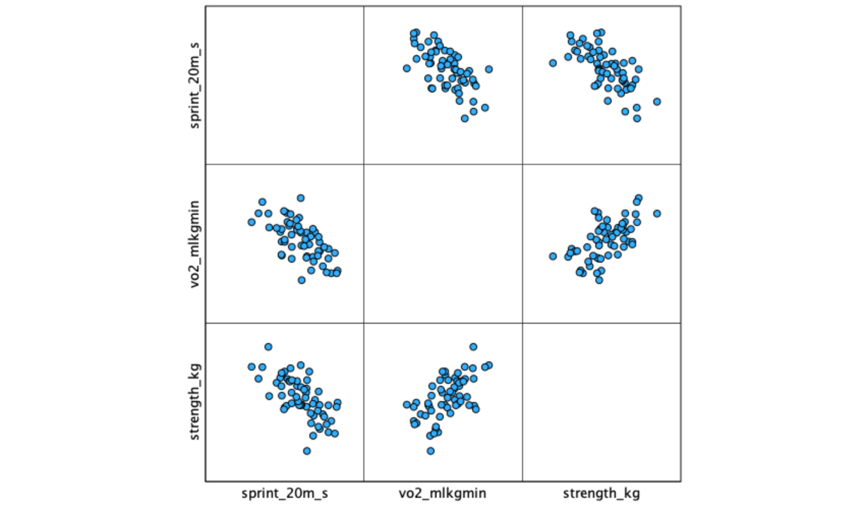
Z.3.2 Interpreting the scatterplot matrix

The matrix produces a grid of scatterplots — each cell shows the relationship between one pair of variables. Examine each panel for:

Direction: Positive or negative trend?
Linearity: Are points roughly following a straight line?
Spread: Is the vertical spread relatively consistent (homoscedasticity)?
Outliers: Any points far from the main cluster?

Pay particular attention to the predictor-predictor panel (vo2_mlkgmin vs. strength_kg). A strong relationship between predictors signals potential multicollinearity, which can destabilize regression coefficient estimates.

Look at all three pairwise panels

A scatterplot matrix gives you three panels at once: sprint vs. VO₂max, sprint vs. strength, and VO₂max vs. strength. The first two show predictor-outcome relationships (you want clear linear trends). The third shows the predictor-predictor relationship (you want a moderate, not extreme, correlation).

Z.4 Part 2: Computing a correlation matrix

Before running the regression, examine the correlation matrix for all three variables. This confirms the direction and magnitude of predictor-outcome relationships and mathematically flags any concerning predictor-predictor correlations that you may have noticed visually in the matrix scatterplot.

Z.4.1 Procedure

Analyze → Correlate → Bivariate…
Move all three variables to the Variables box:
- sprint_20m_s
- vo2_mlkgmin
- strength_kg
Under Correlation Coefficients, ensure Pearson is checked.
Under Test of Significance, select Two-tailed (default).
Leave Flag significant correlations checked.
Click OK.

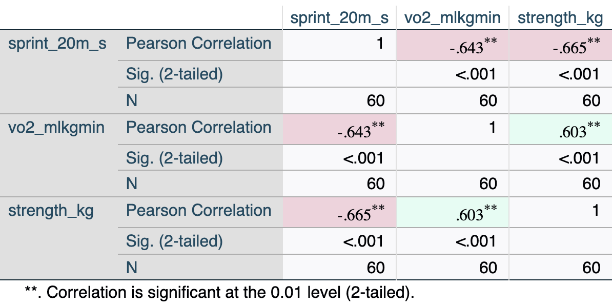
Z.4.2 Interpreting the output

Key elements:

sprint vs. vo2 (\(r\) = −.643): Moderate-to-strong negative relationship — athletes with higher VO₂max tend to have faster sprint times. This is the same relationship examined in the bivariate tutorial.
sprint vs. strength (\(r\) = −.665): Moderate-to-strong negative relationship — stronger athletes tend to sprint faster.
vo2 vs. strength (\(r\) = .603): Moderate positive relationship between predictors — fitter athletes also tend to be stronger. This level of correlation is acceptable; it becomes a concern only above \(|r|\) ≈ .85–.90.

Bivariate \(r^2\) vs. multiple \(R^2\)

In bivariate regression, \(r^2\) equals how much variance the single predictor explains. In multiple regression, the total \(R^2\) will be less than the sum of the two individual \(r^2\) values (\(.414 + .442 = .856\)) because the two predictors share some overlapping variance (they correlate with each other at \(r = .603\)).

Z.5 Part 3: Running multiple linear regression

Z.5.1 Procedure

Analyze → Regression → Linear…
Move sprint_20m_s to the Dependent box.
Move both vo2_mlkgmin and strength_kg to the Independent(s) box.
Leave the Method as Enter (simultaneous entry — all predictors added at once).
Click Statistics…
- ✓ Estimates (regression coefficients) — checked by default
- ✓ Confidence intervals (at 95%)
- ✓ Model fit
- ✓ Descriptives (optional but recommended)
- ✓ Part and partial correlations (shows unique variance for each predictor)
- ✓ Collinearity diagnostics (produces VIF and Tolerance — required for multicollinearity check)
- Continue
Click Plots…
- Move *ZRESID (standardized residuals) to the Y axis.
- Move *ZPRED (standardized predicted values) to the X axis.
- ✓ Check Normal probability plot
- Continue
Click OK.

Method: Enter vs. Stepwise

Leave Method set to Enter for theory-driven research. Avoid stepwise methods (Forward, Backward, Stepwise) — they capitalize on chance variation in the sample and produce models that often fail to replicate. See Chapter 12: Variable Selection Methods for a full discussion.

Z.6 Part 4: Interpreting SPSS output

SPSS produces four main output blocks for multiple regression:

Z.6.1 Descriptive Statistics

The Descriptive Statistics table displays the sample size (\(N\)), mean, and standard deviation for every variable included in the model. This is your first check to ensure the correct variables and cases were processed.

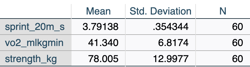
Review the descriptive statistics (Table Z.2) to confirm the data loaded correctly and the filter to time = 'pre' is working (N = 60).

Z.6.2 Model Summary

The Model Summary table provides the overall fit statistics for the model, indicating how well the combination of predictors explains the variance in the outcome variable.

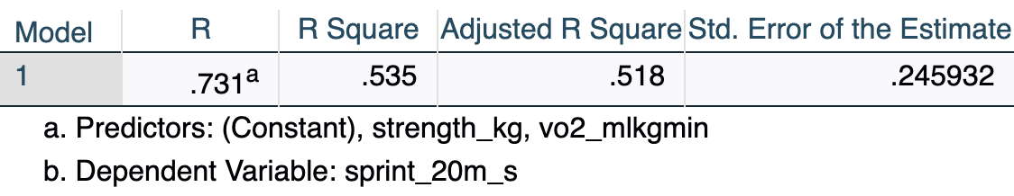
R = .731: The multiple correlation coefficient — the correlation between observed sprint times and those predicted by the full model.
R Square = .535: The two predictors together explain 53.5% of the variance in sprint time.
Adjusted R Square = .518: R² adjusted for sample size (N = 60) and number of predictors (k = 2). This is a more conservative, less biased estimate. It is the preferred value to report in multiple regression.
Std. Error of the Estimate = .246 s: Average distance between observed and predicted sprint times — a measure of prediction accuracy in the original units.

Compare to the bivariate model

In the bivariate tutorial, VO₂max alone explained \(R^2 = .414\) (41.4%) of the variance in sprint time. Adding strength increases this to \(R^2 = .535\) (53.5%) — a gain of 12.1 percentage points of explained variance. Each predictor contributes something unique beyond the other.

Z.6.3 Hypotheses

Multiple regression involves two levels of hypothesis testing. State both before running the analysis.

Omnibus F-test (overall model):

\[H_0: \beta_1 = \beta_2 = 0 \quad \text{(no predictor explains variance in Y)}\] \[H_1: \text{At least one } \beta_i \neq 0\]

Individual predictor t-tests (one per predictor):

For VO₂max (\(X_1\)): \(H_0: \beta_1 = 0\); \(H_1: \beta_1 \neq 0\), controlling for strength.

For Strength (\(X_2\)): \(H_0: \beta_2 = 0\); \(H_1: \beta_2 \neq 0\), controlling for VO₂max.

Z.6.4 ANOVA

The ANOVA (Analysis of Variance) table tests whether the overall regression model is a statistically significant improvement over a baseline model that simply uses the mean of the outcome variable to predict every case.

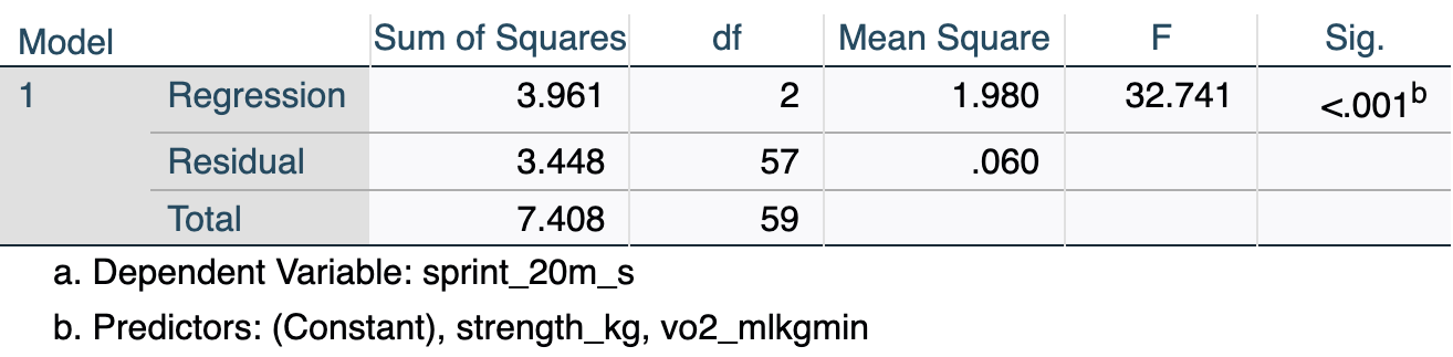
F(2, 57) = 32.74, p < .001: The overall model is statistically significant — together, VO₂max and strength predict sprint time significantly better than simply using the mean sprint time as a prediction for every athlete.
df Regression = 2: One degree of freedom per predictor (k = 2).
df Residual = 57: N − k − 1 = 60 − 2 − 1 = 57.

The omnibus F-test

The ANOVA F-test (Table Z.4) answers: “Does the model as a whole explain a significant amount of variance?” It does not tell you which individual predictors are significant. Use the t-tests in the Coefficients table (Table Z.5) for individual predictor tests.

Z.6.5 Coefficients

The Coefficients table is the core output for multiple regression. It provides the specific estimates (slopes) needed to build the regression equation, significance tests for each individual predictor, and diagnostic statistics like VIF to check for multicollinearity.

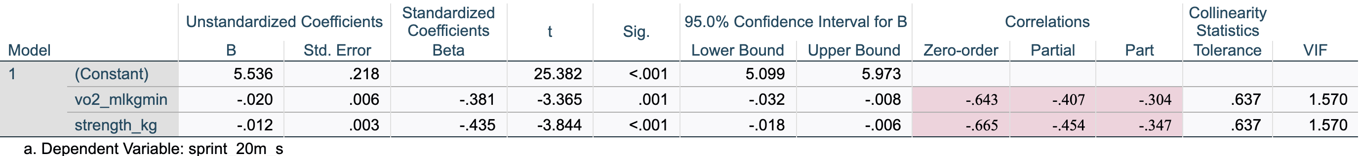
Key values:

Element	Value	Meaning
B (Constant)	5.536	Intercept: predicted sprint time when both predictors = 0 (not meaningful here)
B (vo2_mlkgmin)	−.020	Slope for VO₂max, holding strength constant: each 1 mL·kg⁻¹·min⁻¹ increase in VO₂max is associated with a 0.020 s decrease in sprint time
B (strength_kg)	−.012	Slope for strength, holding VO₂max constant: each additional 1 kg of strength is associated with a 0.012 s decrease in sprint time
Beta (vo2_mlkgmin)	−.381	Standardized slope for VO₂max — allows comparison of effect magnitude across predictors
Beta (strength_kg)	−.435	Standardized slope for strength — larger absolute value than VO₂max, indicating strength has the stronger unique association
Sig. (vo2_mlkgmin)	.001	p = .001 — VO₂max is a significant predictor controlling for strength
Sig. (strength_kg)	.000	p < .001 — strength is a significant predictor controlling for VO₂max
Zero-order	−.643 / −.665	The simple bivariate Pearson correlation (\(r\)) between each predictor and sprint time, ignoring other variables in the model
Partial	−.407 / −.454	The correlation between the predictor and sprint time after removing the effects of other predictors from both variables
Part	−.304 / −.347	The semi-partial correlation: the correlation between the predictor and sprint time after removing the effects of other predictors from the predictor only
VIF	1.57	Well below the threshold of 10 — no multicollinearity concern

The multiple regression equation:

\[\hat{y} = 5.536 + (-0.020) \times \text{VO}_2\text{max} + (-0.012) \times \text{Strength}\]

or equivalently:

\[\hat{y} = 5.536 - 0.020 \times \text{VO}_2\text{max} - 0.012 \times \text{Strength}\]

Why the VO₂max slope changed

In the bivariate model, the VO₂max slope was \(b = -.033\). Here it is \(b = -.020\). The slope decreased in magnitude because part of what VO₂max “did” in the bivariate model was acting as a proxy for strength (the two are correlated at \(r = .603\)). Once strength is included in the model and its effect is accounted for, VO₂max’s unique contribution is smaller. This is normal and expected — it is what “holding constant” means in practice.

Partial vs. Part (Semi-partial) Correlations

When you check Part and partial correlations, SPSS adds three columns to the Coefficients table:

Zero-order: Standard bivariate correlation (from the matrix in Part 2).
Partial: Represents the proportion of unexplained variance in the outcome that is explained by this predictor. For example, holding strength constant, VO₂max explains \((-0.407)^2 = 16.6\%\) of the remaining variance in sprint time.
Part (Semi-partial): Represents the proportion of the total variance in the outcome uniquely explained by this predictor. Squaring this value gives the direct increase in \(R^2\) if this predictor were added last to the model. For example, VO₂max alone accounts for \((-0.304)^2 = 9.2\%\) of the total variance in sprint time.

In multiple regression, the absolute value typically follows this order: Zero-order > Partial > Part.

Z.7 Part 5: Checking assumptions

Multiple regression requires the same assumptions as bivariate regression, plus an additional assumption about multicollinearity. Always evaluate assumptions before interpreting or reporting results.

Assumption checks are built into Part 3

The ZRESID vs. ZPRED residual plot and the Normal P-P plot are requested in the Plots dialog when you run the regression in Part 3 (Steps 6–7). If you followed those steps, SPSS has already generated these plots in the output viewer.

Z.7.1 Assumption 1: Linearity

Check: In the output viewer, locate the Scatterplot of *ZRESID vs. *ZPRED (standardized residuals on the Y-axis, standardized predicted values on the X-axis).

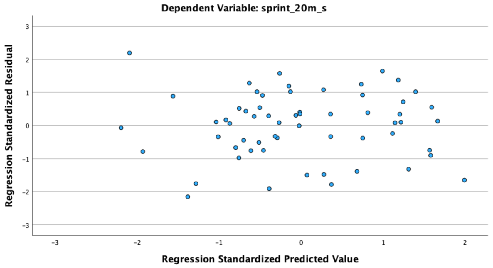
What to look for: Points should scatter randomly around the horizontal zero line with no curved or U-shaped pattern. A systematic curve suggests the linear model is a poor fit and a transformation or polynomial term may be needed.

Z.7.2 Assumption 2: Independence of observations

Check: Study design. When core_session.csv is filtered to time = 'pre', each participant contributes exactly one row — observations are independent. If your own data include repeated measures, clustering, or matched groups, standard regression is not appropriate.

Z.7.3 Assumption 3: Homoscedasticity

Check: Same ZRESID vs. ZPRED plot (Figure Z.2).

What to look for: The vertical spread of points should be roughly constant across all values of ZPRED (no funnel shape). A fan that widens as predicted values increase indicates heteroscedasticity — a violation of the equal-variance assumption.

Z.7.4 Assumption 4: Normality of residuals

Check: In the output viewer, locate the Normal P-P Plot of Regression Standardized Residual.

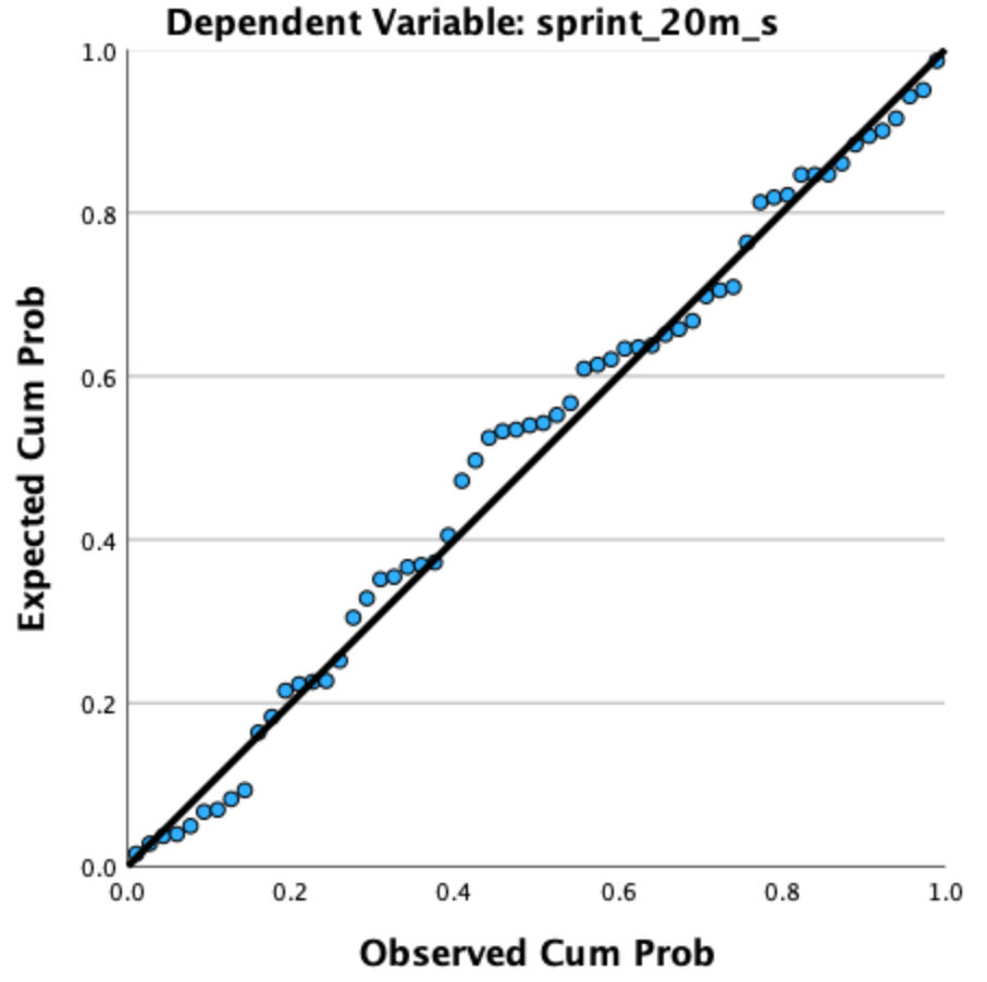
What to look for: Points should fall approximately along the diagonal reference line. Pronounced S-curves or systematic bowing away from the line indicates non-normality. Regression is robust to moderate departures, especially with \(n \geq 30\).

Z.7.5 Assumption 5: No multicollinearity

Check: Use the VIF (Variance Inflation Factor) and Tolerance values from the Coefficients table (Table Z.5). These are produced automatically when you check Collinearity diagnostics in the Statistics dialog (Part 3, Step 5).

Guidelines:

VIF < 5: No problem (VIF = 1.57 for both predictors in this example — well within range)
VIF 5–10: Moderate concern; interpret with caution
VIF > 10: Serious multicollinearity — coefficients may be unstable and standard errors inflated

Tolerance = 1/VIF (= .637 here). Tolerance < .10 indicates a serious problem.

VIF is automatic

SPSS reports VIF whenever you check Collinearity diagnostics under Statistics. Always request it — it is a required diagnostic for multiple regression and should be reported alongside the coefficients.

Z.7.6 Assumption 6: No extreme outliers or influential points

Check: Inspect the ZRESID vs. ZPRED plot for any points far from the main cluster (standardized residuals beyond ±3 are cause for investigation). To formally check influence, save Cook’s Distance:

Z.7.6.1 Procedure: Save Cook’s Distance

Analyze → Regression → Linear…
Re-specify the same model (or run before clicking OK the first time).
Click Save…
- Under Distances, check ✓ Cook’s
- Continue
Click OK.

SPSS adds a new column (COO_1) to your data file. Switch to Data View and sort by COO_1 descending. Values > 1 warrant closer inspection — check whether those participants have data entry errors or are legitimate extreme scores.

Cook’s Distance rule of thumb

Cook’s Distance combines both the size of the residual and the leverage of the case. Most values will be small (< 0.5). Values > 1 are considered influential and should be reported and investigated, not automatically deleted.

Z.8 Part 6: Making predictions

Using the regression equation:

\[\hat{y} = 5.536 - 0.020 \times \text{VO}_2\text{max} - 0.012 \times \text{Strength}\]

Example: Predict 20-m sprint time for an athlete with a VO₂max of 45 mL·kg⁻¹·min⁻¹ and a strength score of 80 kg:

\[\hat{y} = 5.536 - 0.020 \times 45 - 0.012 \times 80 = 5.536 - 0.900 - 0.960 = 3.676 \approx 3.68 \text{ s}\]

Compare to the bivariate prediction: Using only VO₂max (the bivariate model from the previous tutorial), the prediction for the same athlete was \(\hat{y} = 5.174 - 0.033 \times 45 = 3.69\) s. The multiple regression model refines this estimate by also accounting for the athlete’s strength (predicted = 3.68 s).

Both predictor values (VO₂max = 45, Strength = 80) fall within the observed ranges in this dataset, so this is a valid prediction. Avoid using the equation for values outside the observed data range.

In SPSS, you can also save predicted values for all participants:

Analyze → Regression → Linear → Save…
✓ Check Unstandardized Predicted Values
Continue → OK

SPSS adds a new column (PRE_1) to your data file with the model-predicted value for each case.

Z.9 Part 7: Reporting results in APA style

Z.9.1 Sample write-up

A multiple linear regression was conducted to examine whether aerobic capacity (VO₂max) and lower-body strength jointly predicted 20-meter sprint time in collegiate athletes (N = 60, pre-training). The overall model was statistically significant, \(F(2, 57) = 32.74\), \(p < .001\), \(R^2 = .535\), adjusted \(R^2 = .518\), indicating that the two predictors together explained 53.5% of the variance in sprint time (51.8% after adjusting for model complexity). Both predictors made significant unique contributions: VO₂max (\(b = -0.020\), 95% CI \([-0.032, -0.008]\), \(\beta = -.381\), \(p = .001\)) and lower-body strength (\(b = -0.012\), 95% CI \([-0.018, -0.006]\), \(\beta = -.435\), \(p < .001\)). The magnitude of the standardized coefficients indicated that strength had the slightly stronger unique association with sprint time. No multicollinearity concerns were identified (VIF = 1.57 for both predictors).

Z.9.2 APA formatting rules for multiple regression

Report the omnibus \(F\)-test with both degrees of freedom: \(F(2, 57) = 32.74\)
Report both \(R^2\) and adjusted \(R^2\) — the adjusted value is preferred as the primary summary statistic
Report unstandardized (\(b\)) and standardized (\(\beta\)) coefficients for each predictor
Include 95% confidence intervals for each \(b\)
Report VIF values to document that multicollinearity was checked (e.g., VIF = 1.57)
Use p < .001 when SPSS displays .000; use exact p-values otherwise (e.g., \(p = .001\))
Report results for each predictor in a table when there are more than two predictors

Z.9.3 Regression table format (optional)

For papers with multiple predictors, a table is cleaner than inline text:

Table Z.6: Multiple Regression Results

Predictor	\(b\)	95% CI	\(SE\)	\(\beta\)	\(t\)	\(p\)	VIF
Constant	5.536	[5.099, 5.973]	.218		25.38	< .001
VO₂max	−.020	[−.032, −.008]	.006	−.381	−3.37	.001	1.57
Strength	−.012	[−.018, −.006]	.003	−.435	−3.84	< .001	1.57

Note. \(R^2 = .535\); Adjusted \(R^2 = .518\); \(F(2, 57) = 32.74\), \(p < .001\).

Z.10 Part 8: Common mistakes and troubleshooting

Z.10.1 Mistake 1: Not checking multicollinearity

Problem: Running multiple regression and reporting coefficients without evaluating VIF. When predictors are highly intercorrelated, standard errors are inflated and coefficients become unstable — small changes in the sample can produce very different slope estimates.

Solution: Always request Collinearity diagnostics in the Statistics dialog. Report VIF for each predictor. If VIF > 10, consider dropping one of the near-redundant predictors, combining them, or reconsidering the model.

Z.10.2 Mistake 2: Confusing \(b\) (unstandardized) with \(\beta\) (standardized)

Problem: Reporting “\(\beta = -.020\)” or using unstandardized coefficients to compare the relative importance of predictors measured in different units.

Solution: Use \(b\) (unstandardized) for the regression equation, predictions, and reporting the literal effect size in context. Use \(\beta\) (standardized) only to compare the relative contribution of predictors within the same model when they are on different measurement scales.

Z.10.3 Mistake 3: Interpreting each slope as if it were bivariate

Problem: Saying “VO₂max predicts a 0.020-second decrease in sprint time” without acknowledging the “holding strength constant” qualifier.

Solution: Each slope in multiple regression is a partial coefficient — it represents the unique effect of that predictor after removing the influence of all other predictors in the model. Always include this qualifier: “controlling for strength” or “after adjusting for strength.”

Z.10.4 Mistake 4: Using stepwise selection for theory-driven research

Problem: Using SPSS’s Forward, Backward, or Stepwise method to let the software decide which predictors to include. This capitlizes on sample-specific noise and produces models that often fail to replicate.

Solution: Use Method: Enter (simultaneous entry) and select predictors based on theory and prior research. See Chapter 12: Variable Selection Methods for a full discussion.

Z.10.5 Mistake 5: Reporting only the omnibus F-test

Problem: “The model was significant, \(F(2, 57) = 32.74\), \(p < .001\).” This tells the reader the model works, but not which predictors matter or how large their effects are.

Solution: Always follow the omnibus test with coefficient-level reporting: slopes, standard errors, standardized coefficients, confidence intervals, and significance for each predictor.

Z.10.6 Mistake 6: Over-interpreting \(R^2\) as complete explanation

Problem: “\(R^2 = .535\), so we understand sprint performance.”

Solution: \(R^2 = .535\) means the model explains about half the variance in this sample. The other ~47% is due to predictors not included in the model (technique, motivation, muscle fiber composition, etc.). Report \(R^2\) as a measure of model fit in this sample, not as a claim about causal completeness.

Z.11 Summary

This tutorial demonstrated how to:

Produce a scatterplot matrix to visualize all pairwise relationships among three variables
Compute a full correlation matrix using Analyze → Correlate → Bivariate to assess predictor-outcome and predictor-predictor relationships
Conduct a multiple regression using Analyze → Regression → Linear with two predictors entered simultaneously using Method: Enter
Interpret the Model Summary (\(R\), \(R^2\), Adjusted \(R^2\)), ANOVA (omnibus \(F\)-test), and Coefficients table (partial slopes, standardized coefficients, VIF)
Evaluate multicollinearity using VIF (< 5 = acceptable; > 10 = serious concern)
Check regression assumptions including the additional requirement of no multicollinearity
Make predictions using the full multiple regression equation
Report results following APA guidelines including adjusted \(R^2\) and VIF

Key takeaways from this example (VO₂max + strength predicting 20-m sprint time, N = 60, pre-training):

\(F(2, 57) = 32.74\), p < .001 — the overall model is highly significant
Adjusted \(R^2 = .518\) — the two predictors jointly explain approximately 52% of the variance in sprint time
VO₂max: \(b = -0.020\), \(\beta = -.381\) — a significant unique predictor after controlling for strength
Strength: \(b = -0.012\), \(\beta = -.435\) — the slightly stronger unique predictor after controlling for VO₂max
VIF = 1.57 — no multicollinearity concern despite a moderate predictor correlation of \(r = .603\)
Each slope is now a partial coefficient: it reflects the unique effect of that predictor with the other held constant
Adding strength to the VO₂max model increased \(R^2\) from .414 to .535 (+12.1 percentage points)
Use adjusted \(R^2\) as the primary model fit statistic in multiple regression

Next steps

Practice hierarchical regression: enter predictors in blocks to quantify \(\Delta R^2\) — how much each block adds to the model
Explore models with three or more predictors, keeping the \(N\):\(k\) ratio in mind (at least 10–20 observations per predictor)
Review assumption diagnostics more deeply: leverage values, studentized residuals, and DFFITS for influential-point detection
See Chapter 12 of the textbook for deeper coverage of model building, variable selection, and cross-validation

Z.12 Additional resources

SPSS manuals: IBM SPSS Statistics Base documentation
APA Style (7th ed.): Guidelines for reporting regression results
Textbook website: Download practice datasets and syntax files