Adjusting for baseline differences and improving precision in Movement Science
Tip💻 Analytical Software & SPSS Tutorials
A Note on By-Hand Calculations: The purpose of this book is not to teach tedious by-hand statistical calculations. Modern researchers run these analyses using major software packages. While we provide the underlying equations for conceptual understanding, we strongly recommend relying on software for computation to avoid errors and save time.
Please direct your attention to the SPSS Tutorial: ANCOVA in the appendix for step-by-step instructions on running the analysis, testing the homogeneity of regression slopes assumption, obtaining adjusted means, and interpreting SPSS output!
17.1 Chapter roadmap
Every chapter in this textbook so far has assumed that the groups being compared begin on equal footing — or, in the case of repeated measures designs, that the same individuals are measured across conditions. In reality, participants in movement science research are rarely identical at the start of a study. Even with random assignment, one group may enter a training program slightly stronger, fitter, or more experienced than another. Without accounting for these baseline differences, a post-test comparison confounds the genuine effect of the treatment with whatever pre-existing advantage one group happened to carry into the study.
Analysis of Covariance (ANCOVA) was developed precisely for this situation. It extends the ANOVA framework by incorporating one or more continuous covariates — variables measured before the intervention that are expected to correlate with the outcome — and statistically adjusting the group means to remove that pre-existing variability. The result is a comparison of adjusted means: estimates of what each group’s post-test score would have been if all participants had started at the same baseline level. ANCOVA does not simply subtract the pre-test score; it models the linear relationship between the covariate and the outcome, removes that shared variance from the error term, and produces an F-ratio that reflects the group effect with much greater precision than an unadjusted post-test comparison[1,2].
In movement science, ANCOVA is most commonly applied in pretest–posttest control group designs: studies where participants are assessed before and after an intervention, and the goal is to determine whether the intervention produced a genuine post-test difference once the pre-test starting point is accounted for. A strength and conditioning researcher who randomizes 60 participants to a training group or a control group and then measures strength at both time points is in exactly this situation. The pre-test score is the natural covariate, and ANCOVA uses it to sharpen the estimate of the training effect. This chapter develops ANCOVA from the ground up, connects it to the regression framework of Chapters 11 and 12, and works through a complete example using the core_session.csv dataset.
17.2 Learning objectives
By the end of this chapter, you will be able to:
Explain what ANCOVA does conceptually and why it is used in pretest–posttest research designs.
Describe how incorporating a covariate reduces error variance and adjusts group means.
State and verify the homogeneity of regression slopes assumption.
Distinguish between unadjusted and adjusted group means and interpret what the adjustment represents.
Compute and interpret partial eta-squared and partial omega-squared as effect size measures for ANCOVA.
Recognize common pitfalls in the use of ANCOVA, including the consequences of non-random assignment and Lord’s paradox.
Report ANCOVA results in APA style, including covariate information, adjusted means, and effect sizes.
17.3 Workflow for ANCOVA
Use this sequence when a continuous covariate needs to be controlled:
Confirm the covariate is measured before the intervention (or is otherwise not influenced by group assignment).
Check the covariate–outcome correlation — the higher it is, the more error variance ANCOVA will remove.
Test homogeneity of regression slopes — add a Group × Covariate interaction to the model and verify it is non-significant before proceeding.
Run the ANCOVA using SPSS General Linear Model → Univariate with the covariate specified.
Inspect adjusted means from the Estimated Marginal Means output.
Calculate effect sizes (η²_p and ω²_p) from the SPSS output.
Report results in APA format, including the covariate, the adjusted means, and the effect size.
17.4 What ANCOVA does
17.4.1 The core idea: removing covariate variance from error
In a standard between-subjects ANOVA, the error term (MS_error) contains all of the within-group variability in the outcome — every source of individual differences that was not explained by the group factor. When participants differ substantially in relevant characteristics at baseline, this error term is inflated, reducing statistical power. ANCOVA deflates it by partitioning out the portion of outcome variability that is linearly predictable from the covariate before computing the F-ratio for the group effect.
The process has two simultaneous effects. First, it reduces error variance: if the covariate accounts for 80% of the variability in post-test scores, the error term in the ANCOVA is roughly 80% smaller than in the unadjusted ANOVA — a dramatic improvement in statistical power[1,3]. Second, it adjusts the group means to remove the influence of unequal baseline scores. If the training group happened to start slightly stronger than the control group, the ANCOVA-adjusted training mean is pulled downward and the adjusted control mean is pulled upward until both are expressed as estimates for participants who started at the grand mean of the covariate. The adjusted difference is a fairer, more accurate reflection of the treatment effect.
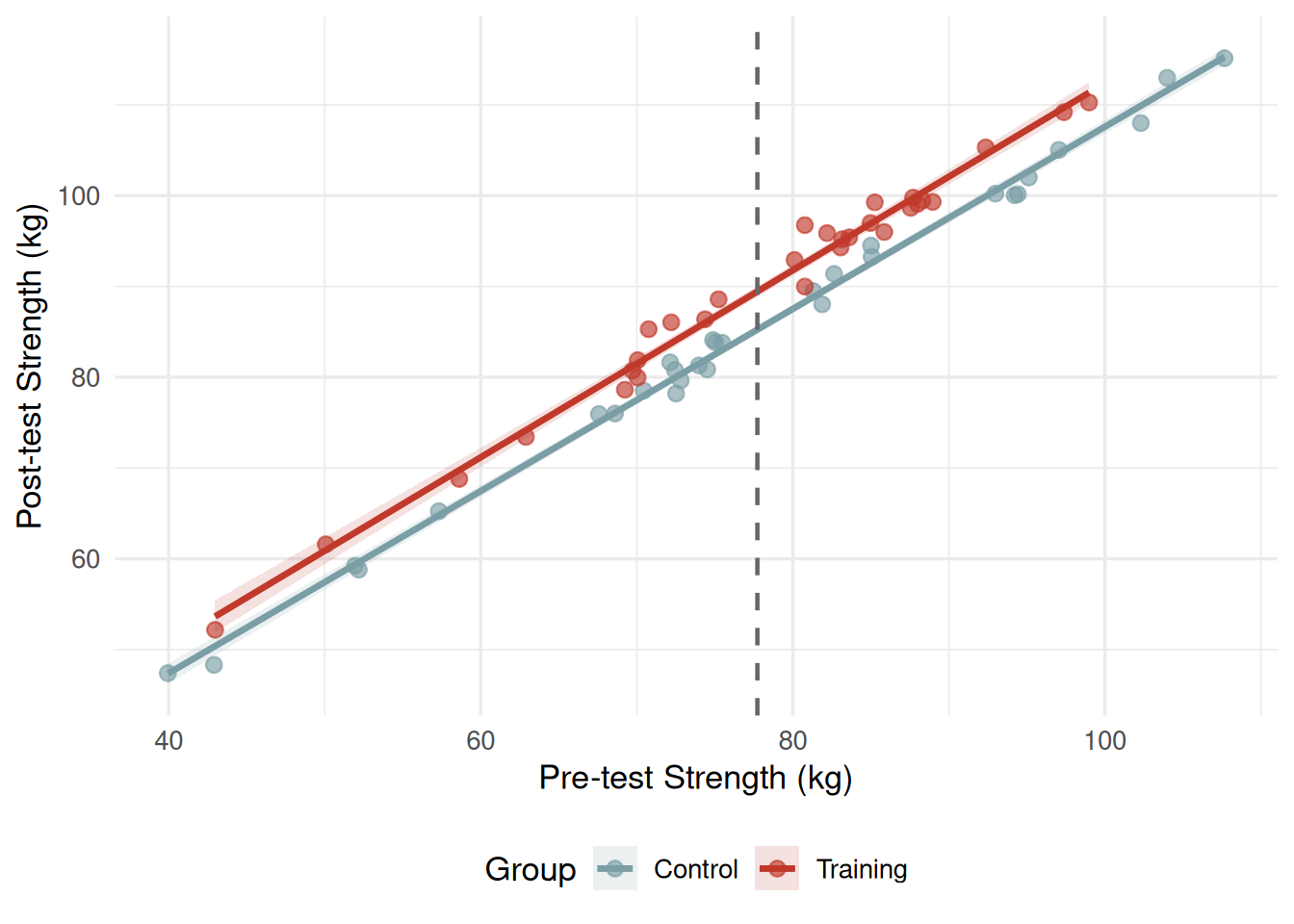
The most intuitive way to understand ANCOVA is through a scatterplot showing the covariate (x-axis) against the outcome (y-axis), with separate points and regression lines for each group. When ANCOVA works well, the two regression lines are approximately parallel — one group’s post-test scores are consistently higher than the other’s by a nearly constant amount, regardless of where participants start on the covariate. The vertical distance between the two parallel lines, measured at the grand mean of the covariate, is the adjusted mean difference — the ANCOVA estimate of the treatment effect. Figure 17.1 illustrates this pattern with the core_session.csv data.
Figure 17.1: Pre-test strength (covariate) vs. post-test strength (outcome) by Group. Each point is one participant. The fitted regression lines are nearly parallel, confirming the homogeneity of regression slopes assumption. The vertical gap between the lines at the grand mean of pre-test strength (dashed vertical line, M = 78.01 kg) represents the ANCOVA-adjusted group difference of 4.53 kg.
17.5 ANCOVA as a regression model
17.5.1 The model equation
ANCOVA is a special case of the general linear model that includes both a categorical predictor (Group) and a continuous predictor (the covariate). For a design with two groups and one covariate, the model is:
where \(Y_i\) is the outcome (post-test strength), \(\text{Group}_i\) is a dummy variable (0 = Control, 1 = Training), \((X_i - \bar{X})\) is the covariate centered at its grand mean (pre-test strength minus the overall mean), and \(\varepsilon_i\) is the residual. The coefficient \(\beta_1\) is the adjusted mean difference — the estimated difference between the two groups at the grand mean of the covariate. The coefficient \(\beta_2\) is the common regression slope, representing how much post-test strength increases for every 1 kg increase in pre-test strength, pooled across both groups.
This connection to regression (Chapters 11 and 12) is important: ANCOVA is not a separate statistical technique but a particular application of the multiple regression framework, using one categorical and one continuous predictor simultaneously. SPSS handles it through the General Linear Model module rather than the Regression module, but the underlying mathematics are identical[2,4].
17.5.2 Adjusted means
The adjusted mean for each group is the predicted value from the ANCOVA model when the covariate is set to its grand mean. If the grand mean pre-test score is \(\bar{X} = 78.01\) kg, then the adjusted mean for the control group is the model’s predicted post-test score for a control participant who started at exactly 78.01 kg — regardless of where the actual control participants started. The formula is:
The covariate term drops out because it is zero when the covariate is at the grand mean. SPSS reports these values automatically in the Estimated Marginal Means table.
17.6 The pretest–posttest design
The pretest–posttest control group design is the most common application of ANCOVA in movement science. Its logic is straightforward: participants are measured on the outcome variable before the intervention (the pre-test, which becomes the covariate), randomly assigned to groups, exposed to the treatment or control condition, and then measured again after the intervention (the post-test, which is the outcome). ANCOVA then tests whether the groups differ on the post-test after statistically removing the variance attributable to the pre-test.
Two benefits work together in this design. The first is error reduction: because pre-test and post-test scores in physical performance are typically highly correlated (often r > .90), incorporating the pre-test as a covariate removes an enormous portion of the residual variance, yielding a much smaller error term and substantially greater statistical power than a simple post-test t-test[1]. The second is mean adjustment: even with random assignment, groups may end up with somewhat different baseline averages by chance, particularly in small samples. ANCOVA adjusts for this, producing a fairer group comparison.
NoteReal example: Correcting for a baseline advantage
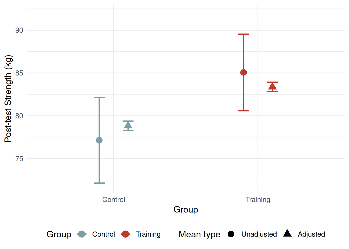
In the core_session.csv dataset, the training group averaged 79.67 kg at pre-test while the control group averaged 76.34 kg — a 3.33 kg baseline difference despite nominal random assignment. An unadjusted post-test comparison would attribute part of the training group’s post-test advantage to this pre-existing difference rather than to the training itself. ANCOVA removes the confound: the adjusted difference of 4.53 kg reflects how much the training group exceeded the control group if both had started at the same strength level (78.01 kg, the grand mean). Because the training group had the baseline advantage, their adjusted mean (83.37 kg) is slightly lower than their unadjusted mean (85.06 kg), while the control group’s adjusted mean (78.83 kg) is slightly higher than their unadjusted mean (77.14 kg).
17.7 Assumptions of ANCOVA
ANCOVA shares the standard ANOVA assumptions — independence of observations, approximate normality of residuals, and homogeneity of variance across groups — and adds two covariate-specific requirements.
17.7.1 Linearity
The relationship between the covariate and the outcome must be approximately linear within each group. If the relationship is curved, the ANCOVA model will misestimate adjusted means and the error reduction will be incomplete. Check linearity by inspecting the scatterplot (such as Figure 17.1) for each group separately. In most pretest–posttest designs with physical performance outcomes, linearity holds well because the same construct is measured at both time points.
17.7.2 Homogeneity of regression slopes
The most important assumption unique to ANCOVA is homogeneity of regression slopes: the slope of the covariate–outcome regression line must be approximately equal across all groups. Visually, this means the regression lines in Figure 17.1 should be parallel. If the slopes differ substantially between groups — if pre-test strength predicts post-test strength more strongly in the training group than in the control group, for example — then a single common slope is a poor model, and the adjusted means will be inaccurate estimates of the true group differences at the grand mean of the covariate.
The homogeneity of slopes assumption is tested by adding a Group × Covariate interaction term to the ANCOVA model. If this interaction is statistically significant, the assumption is violated and standard ANCOVA should not proceed. The data from our training study pass this test comfortably: the Group × Pre-test interaction was F(1, 56) = 0.09, p = .769, indicating that the two groups’ regression slopes (Control b = 1.017, Training b = 1.008) are nearly identical. When the assumption is violated, alternatives include the Johnson–Neyman technique (which identifies regions of the covariate where groups do and do not differ significantly) or separate within-group regressions[1].
WarningCommon mistake: Testing homogeneity of slopes after running the ANCOVA
Homogeneity of regression slopes is a prerequisite for ANCOVA, not an optional diagnostic to run afterward. In SPSS, the slopes test is performed by temporarily adding a Group × Covariate interaction to the model before the main analysis, checking for significance, and then removing the interaction before running the final ANCOVA. If you skip this step and the assumption is violated, the adjusted means in your output are computed from a model that poorly describes the data. See the SPSS Tutorial: ANCOVA for the exact sequence of steps.
17.7.3 Independence of the covariate and the treatment
A critical but often overlooked condition for valid ANCOVA is that the covariate must not be influenced by the treatment. In a pretest–posttest design, using the pre-test score as the covariate satisfies this condition automatically — the pre-test is measured before the treatment begins, so it cannot have been affected by the intervention. Problems arise when researchers try to use a covariate that was measured during or after the treatment period (for example, using midpoint scores as covariates in an ANCOVA of post-test scores), which can produce seriously biased results[5].
17.8 Worked example: Group effect on post-test strength, controlling for pre-test
Research question: After statistically controlling for pre-test strength, is there a significant difference in post-test strength between the training and control groups?
Design: One-way ANCOVA, one between-subjects factor (Group: Control, Training), one covariate (pre-test strength_kg), outcome = post-test strength_kg, N = 60.
Table 17.1: Unadjusted and ANCOVA-adjusted means for post-test strength (kg). Adjusted means are estimated at the grand mean of the covariate (M_pre = 78.01 kg).
Group
Pre-test M (SD)
Post-test M (SD)
Adjusted Post-test M
Control
76.34 (13.70)
77.14 (13.98)
78.83
Training
79.67 (12.26)
85.06 (12.48)
83.37
Grand mean
78.01 (13.01)
81.10 (13.55)
—
Step 1 — Homogeneity of regression slopes test: Before running the ANCOVA, the Group × Pre-test interaction was added to the model. The result was F(1, 56) = 0.09, p = .769 — non-significant. The assumption is met; parallel lines are a reasonable description of the data.
Table 17.2: ANCOVA summary table: Group effect on post-test strength controlling for pre-test strength.
Source
SS
df
MS
F
p
η²_p
Covariate (Pre-test)
27,225.35
1
27,225.35
11,686.00
< .001
.995
Group
303.18
1
303.18
130.18
< .001
.695
Error
132.82
57
2.33
Total
31,676.05
59
Interpretation: After controlling for pre-test strength, the training group (M_adj = 83.37 kg) scored significantly higher than the control group (M_adj = 78.83 kg) at post-test, F(1, 57) = 130.18, p < .001, η²_p = .695 — a large effect. The adjusted mean difference of 4.53 kg reflects the training program’s genuine contribution to strength gains, independent of the groups’ baseline difference.
Notice what ANCOVA accomplished here: the unadjusted post-test t-test yielded t = 2.31, p = .024, while the ANCOVA F-ratio was 130.18 — an enormous gain in precision. This improvement came from two sources. The pre-test covariate explains nearly all of the within-group variability in post-test scores (η²_p = .995 for the covariate; the pre-post correlation was r = .980), so MS_error dropped from approximately 180 kg² in the unadjusted ANOVA to just 2.33 kg² in the ANCOVA — a 99% reduction in error variance. At the same time, the group effect was slightly smaller in the adjusted analysis (4.53 vs. 7.91 kg) because the baseline advantage of the training group was removed.
Figure 17.2: Unadjusted post-test means and ANCOVA-adjusted means (± 95% CI) by Group. The adjustment shifts the training group’s mean downward and the control group’s mean upward, reflecting the removal of the 3.33 kg baseline difference. Both adjusted means are expressed at the grand mean pre-test value of 78.01 kg.
17.9 Interpreting adjusted means
17.9.1 What “controlling for the covariate” really means
Students sometimes describe adjusted means as “removing” or “subtracting” the covariate — as if ANCOVA simply deducts each participant’s pre-test score from their post-test. This is not correct. What ANCOVA does is estimate what each group’s average post-test score would have been if all participants had started at the same covariate value (the grand mean). The adjustment magnitude depends on two things: how much the group’s mean covariate differs from the grand mean, and how strongly the covariate predicts the outcome (the slope b). Groups whose covariate means are close to the grand mean will have adjusted means very similar to their unadjusted means; groups with larger covariate deviations will show larger adjustments[1].
17.9.2 When do adjusted and unadjusted comparisons tell different stories?
In a perfectly balanced randomized experiment with truly equal group means on the covariate, ANCOVA and an unadjusted post-test comparison will yield the same adjusted means — but ANCOVA will still be more powerful, because the error variance is smaller. The adjusted and unadjusted means diverge when groups differ at baseline: the group that starts higher is adjusted downward, and the group that starts lower is adjusted upward. If a group’s unadjusted post-test difference appears significant but disappears after ANCOVA adjustment, the pre-test advantage was doing the work, not the treatment. Conversely, if ANCOVA reveals a significant group difference that was not apparent in the unadjusted comparison, the pre-test disadvantaged the treatment group and was masking the genuine effect. Reporting both unadjusted and adjusted means, as in Table 17.1, gives readers the full picture.
17.10 Effect sizes for ANCOVA
17.10.1 Partial eta-squared and partial omega-squared
Effect size reporting for ANCOVA follows the same partial approach introduced in Chapters 14–16. SPSS reports η²_p automatically for the Group effect and the covariate. For the Group effect:
In our example: η²_p = 303.18 / (303.18 + 132.82) = .695. This is a very large effect — over two-thirds of the residual variance (after removing the covariate) is attributable to the group difference.
As with all ANOVA-family analyses, ω²_p provides a less biased estimate and is preferred for publication. Use the Statistical Calculators appendix or SPSS 31+ to obtain ω²_p from the SS and MS values in the output table.
17.10.2 Cohen’s d for the adjusted difference
For two-group ANCOVA, an interpretable standardized effect size is Cohen’s d for the adjusted mean difference, using the square root of MS_error (the ANCOVA error mean square) as the standardizer:
For our example: \(d_{\text{adj}} = 4.53 / \sqrt{2.33} = 4.53 / 1.53 = \mathbf{2.96}\) — a very large adjusted effect. This standardized difference is directly comparable to Cohen’s d from a paired comparison and reflects the precision gained by removing nearly all of the baseline variance from the error term.
17.11 Sample size and power for ANCOVA
One of ANCOVA’s greatest practical advantages is power. Because the covariate removes a proportion of error variance equal to approximately \(r^2\) — where r is the covariate–outcome correlation — the effective sample size for ANCOVA is larger than for the equivalent ANOVA. When r = .98 (as in our example), \(r^2 = .96\): 96% of the within-group variance is removed from the error term. The required sample size to achieve equivalent power is dramatically reduced.
For power planning in GPower, use F-test: ANOVA: Fixed effects, special, main effects and interactions. The key inputs are the effect size f* (computed from η²_p as \(f = \sqrt{\eta^2_p / (1 - \eta^2_p)}\)), the alpha level, the desired power, and the numerator df (= 1 for two groups). The degrees of freedom for the denominator are reduced by one for each covariate (from N − k to N − k − c where c is the number of covariates), so GPower’s sample size estimate should be increased by c* to account for this. Alternatively, the SPSS 31 power analysis module handles ANCOVA directly.
TipThe stronger the covariate, the bigger the power gain
The power advantage of ANCOVA over ANOVA is directly proportional to \(r^2\) — the squared correlation between the covariate and the outcome. A covariate correlated at r = .50 with the outcome reduces error variance by 25%, providing a modest power boost. A covariate correlated at r = .90 reduces error by 81% — a transformation so powerful that a study requiring n = 100 per group without the covariate might need only n = 20 per group with it. This is why pre-test scores make ideal ANCOVA covariates in movement science: they correlate extremely highly with post-test scores on the same physical performance test, routinely yielding r ≥ .90.
17.12 Reporting ANCOVA in APA style
17.12.1 Template
A one-way ANCOVA was conducted to examine the effect of [Factor] on [outcome], controlling for [covariate]. The assumption of homogeneity of regression slopes was satisfied, F(1, df) = [value], p = [value]. After controlling for [covariate], there was a significant effect of [Factor], F(1, df) = [value], p = [value], η²_p = [value], ω²_p = [value]. The [Group A] group (M_adj = [value], SE = [value]) scored significantly [higher/lower] than the [Group B] group (M_adj = [value], SE = [value]).
17.12.2 Full APA example
A one-way ANCOVA was conducted to examine the effect of training group (control, training) on post-test muscular strength (kg), with pre-test strength as the covariate. Levene’s test indicated homogeneity of error variance, F(1, 58) = 0.12, p = .731. The homogeneity of regression slopes assumption was verified prior to analysis; the Group × Pre-test interaction was non-significant, F(1, 56) = 0.09, p = .769, indicating that the regression slopes relating pre-test to post-test strength were parallel across groups (Control b = 1.02, Training b = 1.01). After adjusting for pre-test strength (b = 1.01, p < .001), there was a significant effect of Group on post-test strength, F(1, 57) = 130.18, p < .001, η²_p = .695. The training group (M_adj = 83.37 kg, SE = 0.28) demonstrated significantly greater post-test strength than the control group (M_adj = 78.83 kg, SE = 0.28), adjusted mean difference = 4.53 kg.
17.13 Common pitfalls and best practices
17.13.1 Pitfall 1: Using ANCOVA to “fix” non-random assignment
ANCOVA is not a remedy for a weak research design. When groups are not randomly assigned — when, for example, self-selected volunteers are compared to a convenience control group — pre-existing differences in the covariate may reflect systematic selection bias rather than random variation. Adjusting for the covariate in this situation can produce severely misleading adjusted means: a group that self-selected into training because they were already motivated, experienced, and physiologically advantaged will differ from the control group on many unmeasured variables, not just the one covariate you adjusted for. ANCOVA controls for one measured covariate; it cannot control for unmeasured confounds[1,5].
17.13.2 Pitfall 2: Lord’s paradox
Lord’s paradox refers to a situation in which two legitimate but different analyses of the same pretest–posttest data yield opposite conclusions about group differences — one analysis (comparing change scores) finds no effect, while another (ANCOVA adjusting for the pre-test) finds a significant effect, or vice versa. This is not a statistical error but a substantive ambiguity: the two analyses answer genuinely different questions. The change-score analysis asks “did the groups change by different amounts?” while ANCOVA asks “do the groups differ at post-test given equal baselines?” When groups start at different baseline levels, these questions have different answers because they involve different counterfactuals[5,6]. The appropriate analysis depends on the research question: if you want to know about the effect of treatment on individuals who happened to be assigned to that treatment, ANCOVA is generally preferred; if you want to know about change in a broader sense, change scores or a mixed ANOVA (Chapter 16) may be more appropriate.
17.13.3 Pitfall 3: Skipping the homogeneity of slopes test
As noted in the Assumptions section, running ANCOVA without first verifying homogeneity of regression slopes risks reporting adjusted means that are computed from a misspecified model. Always run the slopes test as Step 1. If it is significant, consult a statistician or consider alternative approaches (Johnson–Neyman technique, separate within-group regressions) rather than proceeding with standard ANCOVA.
17.13.4 Pitfall 4: Interpreting the covariate’s F-ratio as a group comparison
SPSS always reports an F-ratio for the covariate in the ANCOVA output (in our example, F = 11,686.00 for pre-test strength). This represents the linear relationship between the covariate and the outcome pooled across groups — it is not a group comparison and should not be reported as one. Readers and reviewers may misinterpret a large covariate F as evidence that the covariate “caused” something. Simply state the covariate was significant and report the slope b and its confidence interval.
17.13.5 Pitfall 5: Using multiple covariates without justification
Each covariate added to an ANCOVA model costs one degree of freedom from the error term. Adding a covariate that is weakly correlated with the outcome (r < .30) provides negligible error reduction while shrinking the error df, potentially decreasing rather than increasing power. Include covariates only when there is a strong theoretical reason to expect them to correlate substantially with the outcome, and verify this empirically before the main analysis[2,4].
17.14 Chapter summary
Analysis of Covariance extends the ANOVA framework by incorporating a continuous covariate — typically a pre-test measure of the same or a related outcome — into the model. ANCOVA achieves two simultaneous goals: it adjusts group means to express what each group’s average outcome would have been if all participants had started at the same baseline value, and it removes the covariate’s contribution from the error term, often dramatically improving statistical power. In pretest–posttest designs with high covariate–outcome correlations, ANCOVA can reduce error variance by 80–99%, transforming a modestly powered post-test comparison into a highly sensitive analysis[1,3].
The worked example in this chapter demonstrated both effects clearly. The unadjusted post-test comparison between training and control groups yielded a difference of 7.91 kg with modest statistical significance (t = 2.31); the ANCOVA-adjusted comparison yielded a more honest difference of 4.53 kg with dramatically greater precision (F = 130.18, η²_p = .695), because the pre-test covariate (r = .98 with post-test) accounted for nearly all within-group variability. The adjustment itself was substantively important: the training group had started 3.33 kg stronger at baseline, and ANCOVA correctly attributed part of their raw post-test advantage to this pre-existing difference rather than to the training program.
ANCOVA is a powerful tool, but it carries assumptions that must be explicitly verified — above all, homogeneity of regression slopes — and limitations that must be understood. It does not rescue non-randomized designs from confounding, it cannot adjust for unmeasured variables, and it addresses a different scientific question from a change-score analysis of the same data. Used correctly, within the context of a properly randomized experiment and a well-measured pre-test covariate, ANCOVA is one of the most efficient and informative analytical tools available in movement science research. Chapter 18 moves from designed experiments into reliability analysis, addressing the question of how consistently a measurement instrument performs when applied repeatedly to the same participants — the foundation on which all subsequent inference rests.
17.15 Key terms
analysis of covariance (ANCOVA); covariate; adjusted means; unadjusted means; homogeneity of regression slopes; pretest–posttest design; regression slope; error variance reduction; Johnson–Neyman technique; Lord’s paradox; partial eta-squared; partial omega-squared; Cohen’s d adjusted; common regression slope
17.16 Practice: quick checks
The two simultaneous benefits are error variance reduction and mean adjustment. Error variance reduction occurs because the covariate accounts for a portion of the within-group variability in the outcome — variability that was previously lumped into the error term and suppressed the F-ratio. The amount of reduction is approximately proportional to \(r^2\), the squared correlation between the covariate and the outcome; when \(r\) = .98, as in our strength example, this reduction is nearly total. Mean adjustment occurs because groups rarely have exactly equal covariate means even after random assignment; ANCOVA re-expresses each group’s mean outcome as an estimate of what it would have been if all groups had started at the grand mean of the covariate, producing a fairer comparison of the treatment effect.
The training group entered the study with a 3.33 kg pre-test advantage over the control group (79.67 kg vs. 76.34 kg). Part of their larger post-test mean therefore reflects this pre-existing difference — participants who start stronger tend to end stronger, regardless of training. ANCOVA removes this confound by asking: “If both groups had started at the grand mean of 78.01 kg, how much would the training group still have exceeded the control group?” The answer is 4.53 kg — a smaller number that more accurately captures the genuine effect of the training program. Reporting only the unadjusted difference would overstate the training benefit because it partially reflects luck in group assignment, not the intervention’s true efficacy.
ANCOVA assumes a single common regression slope describes how the covariate relates to the outcome in all groups. If this assumption holds, the within-group regression lines are approximately parallel and the ANCOVA model accurately represents the data. A violation means the slope differs substantially between groups — the covariate may be a strong predictor of post-test scores in the training group but a weak predictor in the control group, for example. In this case, the adjusted means computed by ANCOVA are misleading: they assume a constant gap between the group lines at every value of the covariate, when in reality the gap varies. Visually, a violation appears as crossing or noticeably non-parallel regression lines in the scatter plot. Statistically, the Group × Covariate interaction test in SPSS detects this: a significant result indicates the assumption is violated and standard ANCOVA should not be used.
ANCOVA adjusts for the one covariate that was measured and included in the model, but it cannot adjust for unmeasured pre-existing differences between groups. In a randomized experiment, the only systematic differences between groups are random fluctuations that ANCOVA can address. In a non-randomized study, groups may differ systematically on motivation, training history, socioeconomic status, health status, and dozens of other variables that were never measured. Adjusting for the pre-test score corrects for the observed baseline difference in strength but leaves all these other confounds intact. The adjusted means in a non-randomized ANCOVA can be seriously biased in ways that are difficult to detect. ANCOVA is a tool for improving precision in randomized designs, not a substitute for randomization.
Best practice is to report both, as demonstrated in Table 17.1. Unadjusted means describe the actual observed data and allow readers to situate the sample relative to normative values or other studies. Adjusted means answer the primary inferential question — what is the treatment effect independent of baseline differences? — and should be the focus of the statistical conclusions. When baseline group means are nearly identical (common in large, well-randomized studies), adjusted and unadjusted means are very similar, and reporting both helps readers verify that the ANCOVA adjustment was modest. When baseline means differ substantially, the comparison between adjusted and unadjusted means is itself informative, showing precisely how much of the post-test difference was attributable to pre-existing differences versus the intervention.
Both analyses are statistically correct, but they answer different questions — this is the essence of Lord’s paradox. The change-score analysis asks: “Did the two groups change by different amounts?” The ANCOVA asks: “Do the two groups differ at post-test, given that we equate them on pre-test strength?” When groups start at different baseline levels, these questions can yield different answers. If the treatment group started lower than the control group, their change scores might be large but their adjusted post-test means might not exceed those of the control group — or vice versa. The appropriate analysis depends on the research question and theoretical framework. For most intervention studies in movement science, ANCOVA is preferred because it answers the more relevant question: does treatment produce higher post-test performance than control, accounting for where participants started? However, if the research question is specifically about change (e.g., in a rehabilitation context where the rate of recovery is the focus), change-score analysis may be more appropriate.
NoteRead further
For a thorough treatment of ANCOVA theory and practice, including coverage of assumption violations and alternatives, see[1].[2] provides an in-depth model-comparison perspective that connects ANCOVA to regression.[5] is essential reading on the common misinterpretations of ANCOVA in non-randomized designs, and[6] is the original statement of Lord’s paradox.
NoteNext chapter
Chapter 18 introduces Quantifying Reliability in Movement Science — examining how consistently measurement instruments perform when applied repeatedly to the same participants. Reliability is the statistical foundation beneath all of the inferential procedures in this textbook: a measurement with poor reliability inflates error variance, attenuates correlations, and reduces the power of every analysis covered so far.
1. Huitema, B. E. (2011). The analysis of covariance and alternatives: Statistical methods for experiments, quasi-experiments, and single-case studies (2nd ed.). Wiley.
2. Maxwell, S. E., Delaney, H. D., & Kelley, K. (2018). Designing experiments and analyzing data: A model comparison perspective (3rd ed.). Routledge.
3. Cohen, J. (1988). Statistical power analysis for the behavioral sciences (2nd ed.). Lawrence Erlbaum Associates.
4. Tabachnick, B. G., & Fidell, L. S. (2019). Using multivariate statistics.
5. Miller, G. A., & Chapman, J. P. (2001). Misunderstanding analysis of covariance. Journal of Abnormal Psychology, 110(1), 40–48. https://doi.org/10.1037/0021-843X.110.1.40
6. Lord, F. M. (1967). A paradox in the interpretation of group comparisons. Psychological Bulletin, 68(5), 304–305. https://doi.org/10.1037/h0025105