Comparing three or more group means in Movement Science
Tip💻 Analytical Software & SPSS Tutorials
A Note on By-Hand Calculations: The purpose of this book is not to teach tedious by-hand statistical calculations. Modern researchers run these analyses using major software packages. While we provide the underlying equations for conceptual understanding, we strongly recommend relying on software for computation to avoid errors and save time.
Please direct your attention to the SPSS Tutorial: One-Way ANOVA in the appendix for step-by-step instructions on running ANOVA, checking assumptions, conducting post hoc tests, computing effect sizes, and interpreting output!
14.1 Chapter roadmap
Movement Science researchers frequently need to compare performance or physiological outcomes across more than two groups simultaneously. A coach might ask whether athletes using three different training protocols differ in sprint speed. A clinician might ask whether balance performance varies across four age groups. A researcher might compare VO₂max among sedentary, recreationally active, and trained individuals. In each case, the temptation is to run multiple independent t-tests — one for each pair of groups. However, this approach inflates the probability of falsely rejecting at least one null hypothesis, a problem known as familywise error rate inflation[1,2]. Analysis of Variance (ANOVA) solves this problem by testing whether any group means differ in a single, unified analysis that maintains the stated Type I error rate[3,4].
The logic of ANOVA rests on partitioning variance: the total variability in a dataset is divided into two components — variability between groups (reflecting differences in group means) and variability within groups (reflecting random individual-to-individual differences and measurement error)[2,5]. The F-ratio is formed by dividing between-groups variability by within-groups variability. When the null hypothesis is true and all group means are equal, both components estimate the same population variance, and F ≈ 1. When group means truly differ, between-groups variance is inflated relative to within-groups variance, producing a large F that is unlikely under the null hypothesis[1,3]. This elegant signal-to-noise framework is why ANOVA has been a cornerstone of experimental design in Movement Science for decades[6,7].
This chapter covers one-way between-subjects ANOVA, the simplest and most common form of ANOVA, in which a single independent variable (factor) with three or more levels is used to compare group means on a continuous dependent variable. You will learn when ANOVA is the appropriate choice, how to read and interpret an ANOVA source table, how to check the test’s assumptions, how to use post hoc tests to identify which specific groups differ, and how to quantify the magnitude of group differences using effect sizes. Building on the foundation established in Chapter 13, this chapter extends your ability to design and analyze comparative studies in Movement Science[8,9].
By the end of this chapter, you will be able to:
Explain why ANOVA is preferred over multiple t-tests when comparing three or more groups.
Describe how total variance is partitioned into between-groups and within-groups components.
Interpret an ANOVA source table, the F-statistic, and its associated p-value.
Check assumptions of one-way ANOVA and identify appropriate responses to violations.
Select and apply post hoc tests to identify specific pairwise differences.
Compute and interpret effect sizes (η², ω²) for ANOVA results.
Report one-way ANOVA results in APA format.
14.2 Workflow for one-way ANOVA
Use this sequence whenever you compare means across three or more independent groups:
Identify the research design (one factor with 3+ levels, between-subjects).
State hypotheses (H₀: all population means equal; H₁: at least one mean differs).
Check assumptions (independence, normality within groups, homogeneity of variance).
Run the one-way ANOVA and examine the omnibus F-test.
If F is significant, run post hoc tests to identify which group pairs differ.
Calculate effect sizes (η² or ω²) and confidence intervals.
Interpret and report results in APA format, emphasizing practical significance.
14.3 Why ANOVA exists: the multiple comparisons problem
Suppose a researcher wants to compare jump height across three training groups: plyometric, resistance, and control. To compare all pairs, three independent t-tests would be needed: plyometric vs. resistance, plyometric vs. control, and resistance vs. control. At α = .05, each test carries a 5% chance of a false positive. But with three tests, the probability of committing at least one Type I error rises above 5%[2].
More precisely, the familywise error rate for c independent comparisons is:
\[
\alpha_{\text{FW}} = 1 - (1 - \alpha)^c
\]
With three comparisons at α = .05, the familywise error rate is approximately .14 — nearly three times the intended 5%. With five groups requiring ten pairwise comparisons, it climbs to approximately .40: a 40% chance of at least one false-positive finding[2,4]. Running uncorrected multiple t-tests in place of ANOVA is therefore not merely a stylistic choice — it is a methodological error that produces misleading conclusions.
ANOVA addresses this by testing a single omnibus null hypothesis — that all group means are equal — in one analysis that maintains the stated α level[1]. If the omnibus test is significant, post hoc procedures (covered below) then make pairwise comparisons while controlling the familywise error rate.
WarningCommon mistake: Running multiple t-tests instead of ANOVA
When comparing three or more groups, running a separate t-test for each pair inflates Type I error far beyond the stated α level[2]. Always use ANOVA for the omnibus test, then apply appropriate post hoc procedures for pairwise comparisons.
14.4 The logic of ANOVA: partitioning variance
14.4.1 Sources of variance
The central insight of ANOVA is that total variability in the data can be decomposed into two meaningful components[1,3]:
\(SS_{\text{total}}\) = total sum of squares; overall variability of all scores around the grand mean
\(SS_{\text{between}}\) = between-groups sum of squares; variability of group means around the grand mean (reflects the effect of the independent variable)
\(SS_{\text{within}}\) = within-groups sum of squares; variability of individual scores around their group mean (reflects random error and individual differences)
Think of it this way: in a study comparing three training programs, some variability in fitness outcomes reflects genuine differences between programs (which program you were in), and some reflects differences within programs (individuals vary in how they respond to any given program). ANOVA quantifies both and compares them[2,4].
NoteAn Example
Imagine you assign people to one of three training programs (A, B, C) for 8 weeks and measure VO₂ max. ANOVA asks: do the outcome differences reflect the programs, or just random individual variation?
Two sources of variability:
Between‑program — variation explained by which program someone did. If programs differ systematically, group means will be spread apart (e.g., A = 40, B = 45, C = 50). ANOVA calls this the between‑groups sum of squares.
Within‑program — variation among people in the same program. Even within Program A, individuals differ in fitness and adherence, so scores might range 32–48 around a mean of 40. ANOVA calls this the within‑groups (residual/error) sum of squares.
F is large when group means differ more than the noise within groups would predict — evidence the programs have different effects. F near 1 means the group-mean differences are no larger than expected from chance alone.
Two scenarios:
Scenario 1 (F ≈ 1)
Scenario 2 (F large)
Group means
A = 40, B = 41, C = 40.5
A = 35, B = 45, C = 55
Within-group spread
30–50 per group
±2 around each mean
Verdict
Group means differ by ≤1 unit, but individuals within each group vary by ±10 — the between-group signal is tiny compared to the within-group noise → F ≈ 1, p > .05
Group means differ by 10 units, but individuals within each group vary by only ±2 — the signal far exceeds the noise → F is large, p < .05
ANOVA doesn’t simply ask “do the means differ?” — it asks whether the differences are large relative to how much individuals vary within each group.
14.4.2 The ANOVA source table
Results are organized in a source table that displays the decomposition of variance and the test statistic:
Source
SS
df
MS
F
p
Between groups
\(SS_B\)
\(k - 1\)
\(MS_B = SS_B / df_B\)
\(MS_B / MS_W\)
Within groups
\(SS_W\)
\(N - k\)
\(MS_W = SS_W / df_W\)
Total
\(SS_T\)
\(N - 1\)
Where \(k\) = number of groups and \(N\) = total sample size.
Mean squares (MS) are obtained by dividing each SS by its degrees of freedom — converting sums of squares into variance estimates that can be meaningfully compared regardless of sample size[3].
14.4.3 The F-statistic
The F-ratio is the heart of ANOVA:
\[
F = \frac{MS_{\text{between}}}{MS_{\text{within}}}
\]
When H₀ is true (all group means equal), both MS_between and MS_within estimate the same population variance → F ≈ 1
When H₁ is true (at least one mean differs), MS_between is inflated by true group differences → F > 1
Larger F values provide stronger evidence against H₀
The F-statistic follows an F-distribution with numerator degrees of freedom \(df_1 = k - 1\) and denominator degrees of freedom \(df_2 = N - k\). The F-distribution is always positive and right-skewed, and its shape depends on both degrees of freedom[2].
TipThink of F as a signal-to-noise ratio
MS_between captures the “signal” — how much group means differ from each other. MS_within captures the “noise” — how much individuals vary within their own groups. F = signal / noise. A large F means the signal clearly rises above the background noise, supporting rejection of H₀[4].
14.5 One-way ANOVA in practice
14.5.1 When to use one-way ANOVA
One-way between-subjects ANOVA is appropriate whenever a researcher wants to compare group means across three or more groups that are defined by a single categorical independent variable, and where each participant belongs to one and only one group[5–7]. The “one-way” designation refers to the presence of a single factor — for example, training type (endurance, resistance, or control) or age category (young adult, middle-aged, older adult). The “between-subjects” designation means that different participants are in each group rather than the same participants being measured repeatedly; designs involving repeated measurements are addressed in Chapter 15.
The dependent variable must be measured on a continuous scale — interval or ratio — because ANOVA operates on means and variances. Comparing gait speed across three fall-risk groups, jump height across four training protocols, or grip strength across three diagnostic categories would all qualify. If the outcome is ordinal or clearly non-normal with small samples, the nonparametric Kruskal-Wallis test (Chapter 19) is the appropriate alternative[10].
A common source of confusion is whether ANOVA or a t-test is appropriate when exactly three groups are involved. The answer is unambiguous: with three or more groups, ANOVA is required. The independent-samples t-test is restricted to two groups. Even with three groups, running pairwise t-tests instead of ANOVA inflates the familywise error rate as described earlier, making ANOVA not just an option but a methodological necessity[2,4].
NoteReal example: Comparing VO₂max across training groups
A researcher randomly assigns 60 university students to one of three 12-week training programs: endurance training (n = 20), resistance training (n = 20), or a no-exercise control group (n = 20). VO₂max (mL·kg⁻¹·min⁻¹) is measured at post-training. The researcher wants to know whether VO₂max differs across the three groups. With one factor (training group) at three levels and a continuous DV (VO₂max), one-way ANOVA is the appropriate test[5].
All population means are equal — the independent variable has no effect on the dependent variable.
Alternative hypothesis (H₁):
At least one population mean differs from the others.
ImportantH₁ does not specify which groups differ
A significant F-test only tells you that somewhere among the groups there is a difference — it does not identify which group pairs are responsible. Post hoc tests (see below) are required to answer that more specific question[4,11].
14.5.3 Worked example: One-way ANOVA
Using the VO₂max training study described above, the steps to conduct a one-way ANOVA are:
Step 1: State hypotheses
H₀: μ_endurance = μ_resistance = μ_control (training group has no effect on VO₂max)
H₁: At least one training group mean differs
α = .05
Step 2: Check assumptions
Before running the ANOVA, verify that independence, normality, and homogeneity of variance are met (see the Assumptions section below and the SPSS tutorial).
Step 3: Run the ANOVA in SPSS
(See the SPSS Tutorial: One-Way ANOVA for a full walkthrough of the SPSS procedure, output tables, and interpretation steps.)
Step 4: Interpret the source table output
Suppose SPSS produces the following:
Source
SS
df
MS
F
p
Between groups
1,248.6
2
624.3
14.87
< .001
Within groups
2,391.4
57
41.95
Total
3,640.0
59
With F(2, 57) = 14.87, p < .001, we reject H₀ and conclude that VO₂max differs significantly across at least two of the three training groups. Post hoc tests are then needed to identify which specific pairs differ.
Step 5: Compute and report effect size
\(\eta^2 = SS_{\text{between}} / SS_{\text{total}} = 1248.6 / 3640.0 = .343\), indicating a large effect — approximately 34% of the total variance in VO₂max is accounted for by training group assignment[8].
Interpretation
A one-way ANOVA revealed a significant effect of training group on VO₂max, F(2, 57) = 14.87, p < .001, η² = .34. This indicates that at least one training group’s mean VO₂max differed meaningfully from the others. Post hoc comparisons are needed to identify the source of this difference.
14.6 Assumptions of one-way ANOVA
One-way ANOVA rests on three key assumptions[2–4]:
Independence of observations: Scores from different participants are independent. This is ensured by research design (random assignment, no repeated measures). Violations produce serious errors that cannot be corrected statistically.
Normality: The dependent variable is approximately normally distributed within each group. With larger samples (n ≥ 30 per group), ANOVA is robust to moderate departures from normality due to the Central Limit Theorem[12,13].
Homogeneity of variance: Population variances are approximately equal across all groups. This assumption can be tested formally and, when violated, robust alternatives exist.
14.6.1 Checking normality
Normality should be evaluated within each group separately, not across the entire sample pooled together. The most informative initial step is visual inspection: histograms and normal Q-Q plots for each group reveal the shape of the distribution, the presence of extreme outliers, and any floor or ceiling effects that might indicate a non-normal distribution[4]. Q-Q plots are especially useful because departures from normality appear as systematic deviations from a straight diagonal line, making moderate skewness or heavy tails easy to spot even with modest sample sizes.
For a formal statistical test of normality, the Shapiro-Wilk test is the recommended choice because of its superior sensitivity to departures from normality across a wide range of distribution shapes[4]. Modern implementations support samples ranging from as few as 3 to as many as 5,000 observations per group. A non-significant Shapiro-Wilk test (p > .05) supports the normality assumption, though it should be interpreted alongside the visual plots rather than in isolation — with large samples even trivial non-normality will produce significant results, while with very small samples the test has little power to detect meaningful violations.
Fortunately, one-way ANOVA is reasonably robust to moderate departures from normality, particularly when group sizes are approximately equal and sample sizes are at least 30 per group. Under these conditions, the Central Limit Theorem ensures that sampling distributions of group means are approximately normal even if raw scores are not[12,13]. Smaller samples with pronounced skewness or heavy tails warrant greater caution, and a data transformation or nonparametric alternative should be considered in those cases.
14.6.2 Checking homogeneity of variance
The homogeneity of variance assumption is formally evaluated using Levene’s test, which tests the null hypothesis that all population variances are equal: H₀: σ₁² = σ₂² = ⋯ = σₖ²[14]. A non-significant result (p > .05) supports the assumption and licenses use of the standard F-test and Tukey HSD post hoc comparisons. A significant Levene’s test (p < .05) indicates that group variances are sufficiently unequal to warrant a correction; in that case, Welch’s ANOVA or the Brown-Forsythe ANOVA should be used in place of the standard F-test (see the warning callout below). In SPSS, Levene’s test is produced automatically when you check the “Homogeneity of Variance” option under Options in the One-Way ANOVA dialog.
A useful practical rule of thumb is to compare the standard deviations across groups: if the largest group SD is less than twice the smallest group SD, the equal-variance assumption is unlikely to cause meaningful problems in practice, even if Levene’s test is technically significant in large samples[4]. This is because the F-test is moderately robust to mild heteroscedasticity when group sizes are equal or nearly equal. When group sizes are substantially unequal and variances differ, the robustness of the F-test breaks down more sharply, and the corrected tests become important[15].
WarningWhat to do when Levene’s test is significant
When Levene’s test indicates unequal variances (p < .05), use Welch’s ANOVA (also called the Welch F-test) or the Brown-Forsythe ANOVA, both of which adjust for heterogeneous variances[4]. In SPSS, these are available under Analyze → Compare Means → One-Way ANOVA → Options → Welch and Brown-Forsythe. For post hoc comparisons under unequal variances, use the Games-Howell procedure[16].
14.6.3 When assumptions are severely violated
If normality is substantially violated (especially with small samples):
Data transformation: Log or square root transformations may normalize the distribution[17]
Kruskal-Wallis test: The nonparametric alternative to one-way ANOVA; compares ranked scores rather than means (see Chapter 19)[10]
14.7 Post hoc tests
A significant omnibus F-test establishes that at least one group mean differs, but does not identify which pairs of groups are responsible. Post hoc tests make all pairwise comparisons while controlling the familywise error rate[2,11].
ImportantOnly run post hoc tests after a significant F
Post hoc comparisons are only meaningful following a statistically significant omnibus F-test. Running post hoc tests on a non-significant ANOVA result — sometimes called “fishing” — inflates Type I error and produces unreliable conclusions[4].
14.7.1 Choosing a post hoc test
The appropriate post hoc procedure depends on whether the homogeneity of variance assumption is met and whether group sizes are equal[4,16]:
Test
Equal variances?
Equal n?
Characteristics
Tukey HSD
Yes
Preferred
Most widely used; good balance of Type I/II error control
Bonferroni
Yes
Any
Conservative; best when number of comparisons is small
Games-Howell
No
Any
Preferred when Levene’s test is significant
Scheffé
Yes
Any
Very conservative; suited for complex (non-pairwise) comparisons
Recommendation: Use Tukey HSD when assumptions are met. Switch to Games-Howell when Levene’s test is significant[4,16].
14.7.2 Interpreting post hoc output
For the VO₂max example, Tukey HSD post hoc comparisons might reveal:
Comparison
Mean Difference
SE
p (adjusted)
95% CI
Endurance − Resistance
7.2
2.05
.003
[2.1, 12.3]
Endurance − Control
11.8
2.05
< .001
[6.7, 16.9]
Resistance − Control
4.6
2.05
.082
[−0.5, 9.7]
From this output: endurance training produced significantly higher VO₂max than both resistance training and the control group; resistance training did not significantly differ from the control group at α = .05. The 95% CIs confirm the direction and magnitude of each difference.
NoteReal example: Post hoc comparisons in training research
In a study comparing three resistance training protocols (high volume, high intensity, and moderate), a one-way ANOVA found a significant overall effect on 1-RM squat strength, F(2, 45) = 8.34, p < .001. Tukey HSD post hoc tests revealed that high-volume training produced significantly greater strength gains than the moderate protocol (p = .008), but did not significantly differ from high-intensity training (p = .12). Such nuanced comparisons are only possible through proper post hoc procedures following a significant omnibus F[5,18].
14.8 Effect sizes in ANOVA
A significant F-test answers whether groups differ, but not how much they differ. Effect sizes are essential for interpreting practical significance and for planning future studies[8,9,19].
14.8.1 Eta-squared (η²)
Eta-squared is the most commonly reported effect size in ANOVA[20]:
It represents the proportion of total variance in the dependent variable explained by group membership. Benchmarks (Cohen, 1988):
η² = .01: Small effect
η² = .06: Medium effect
η² = .14: Large effect
Limitation: η² slightly overestimates the population effect size, particularly in small samples, because \(SS_{\text{total}}\) includes variability from the factor being estimated[20].
14.8.2 Omega-squared (ω²)
Omega-squared provides a less biased estimate of the population effect size[20]:
ω² is preferred over η² when reporting results, particularly with small-to-moderate samples, because it corrects for the upward bias in η²[9,20]. The same Cohen (1988) benchmarks (.01/.06/.14) are used for interpretation.
14.8.3 Cohen’s f
Cohen’s f is a standardized effect size well suited to power analysis planning[8]:
\[
f = \sqrt{\frac{\eta^2}{1 - \eta^2}}
\]
Benchmarks (Cohen, 1988):
f = .10: Small effect
f = .25: Medium effect
f = .40: Large effect
Cohen’s f is the effect size metric used in G*Power when planning sample sizes for ANOVA[21].
14.8.4 Which effect size to report?
The short answer for published research is to prioritize ω². Because η² systematically overestimates the population effect — it treats the sample’s own variability as the denominator rather than correcting for it — ω²’s penalty for the number of groups and the within-group variance produces an estimate that generalizes more honestly to the broader population[9,20]. This distinction is especially consequential with small-to-moderate total samples, where η² can exceed the true effect by a meaningful margin.
That said, it is worth also reporting η² alongside ω² whenever you are directly comparing your results to existing literature, since the vast majority of published Movement Science studies report η² rather than ω². Providing both values with a brief note that η² is the commonly used but upwardly biased estimate allows readers to interpret your findings relative to the prior literature while still appreciating the more conservative estimate[9,20].
Regardless of which variance-explained effect size you report, always accompany it with 95% confidence intervals when your software provides them. A point estimate alone — whether η² = .34 or ω² = .32 — communicates the sample result but not the precision of that estimate[19]. Wide confidence intervals signal that the true effect could be considerably smaller or larger than observed, which has direct implications for how the findings should be weighted in practice. Finally, when the goal is planning a future study or conducting a power analysis, convert η² or ω² into Cohen’s f using the formula given above. GPower requires Cohen’s f* as its input, and this translation ensures that power calculations are grounded in the same effect size estimate you observed[8,21].
Importantη² overestimates — report ω² for small samples
With small samples (total N < 100), η² can substantially overestimate the true population effect. ω² is a more conservative and honest estimate. Software such as JASP and R’s effectsize package compute both automatically[9,20].
14.9 Visualizing ANOVA results
Effective visualizations help communicate both the central tendency and variability of each group[22,23].
14.9.1 Box plots by group
Code
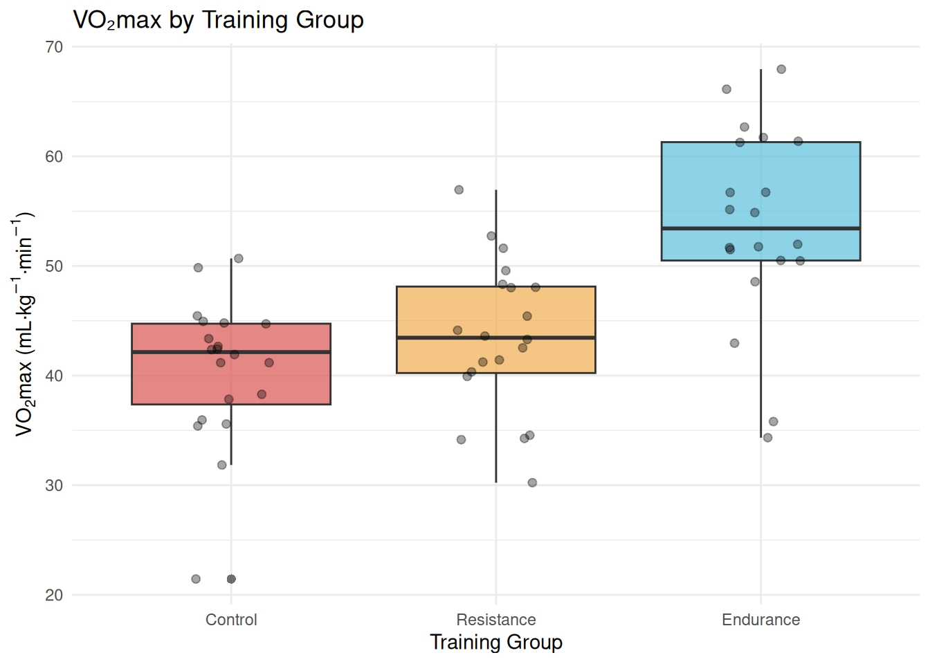
library(ggplot2)set.seed(42)n <-20vo2 <-data.frame(Group =factor(rep(c("Endurance", "Resistance", "Control"), each = n),levels =c("Control", "Resistance", "Endurance")),VO2max =c(rnorm(n, mean =52.4, sd =6.8), # Endurancernorm(n, mean =45.2, sd =6.2), # Resistancernorm(n, mean =40.6, sd =6.4) # Control ))ggplot(vo2, aes(x = Group, y = VO2max, fill = Group)) +geom_boxplot(alpha =0.7, outlier.shape =16, outlier.size =2) +geom_jitter(width =0.15, alpha =0.35, size =1.8) +scale_fill_manual(values =c("Control"="#d9534f","Resistance"="#f0ad4e","Endurance"="#5bc0de")) +labs(x ="Training Group", y =expression(VO[2]*"max (mL·kg"^-1*"·min"^-1*")"),title ="VO₂max by Training Group") +theme_minimal() +theme(legend.position ="none")
Figure 14.1: VO₂max (mL·kg⁻¹·min⁻¹) across three training groups. Box plots display the median, interquartile range, and outliers for each group. Endurance training produced notably higher and more variable VO₂max values compared to resistance and control groups.
Box plots (Figure 14.1) reveal the full distribution of VO₂max scores within each group, making it easy to spot differences in both central tendency and spread. The endurance group shows clearly higher medians and interquartile ranges, consistent with the known aerobic demands of endurance training[5].
14.9.2 Error bar plots with confidence intervals
Code
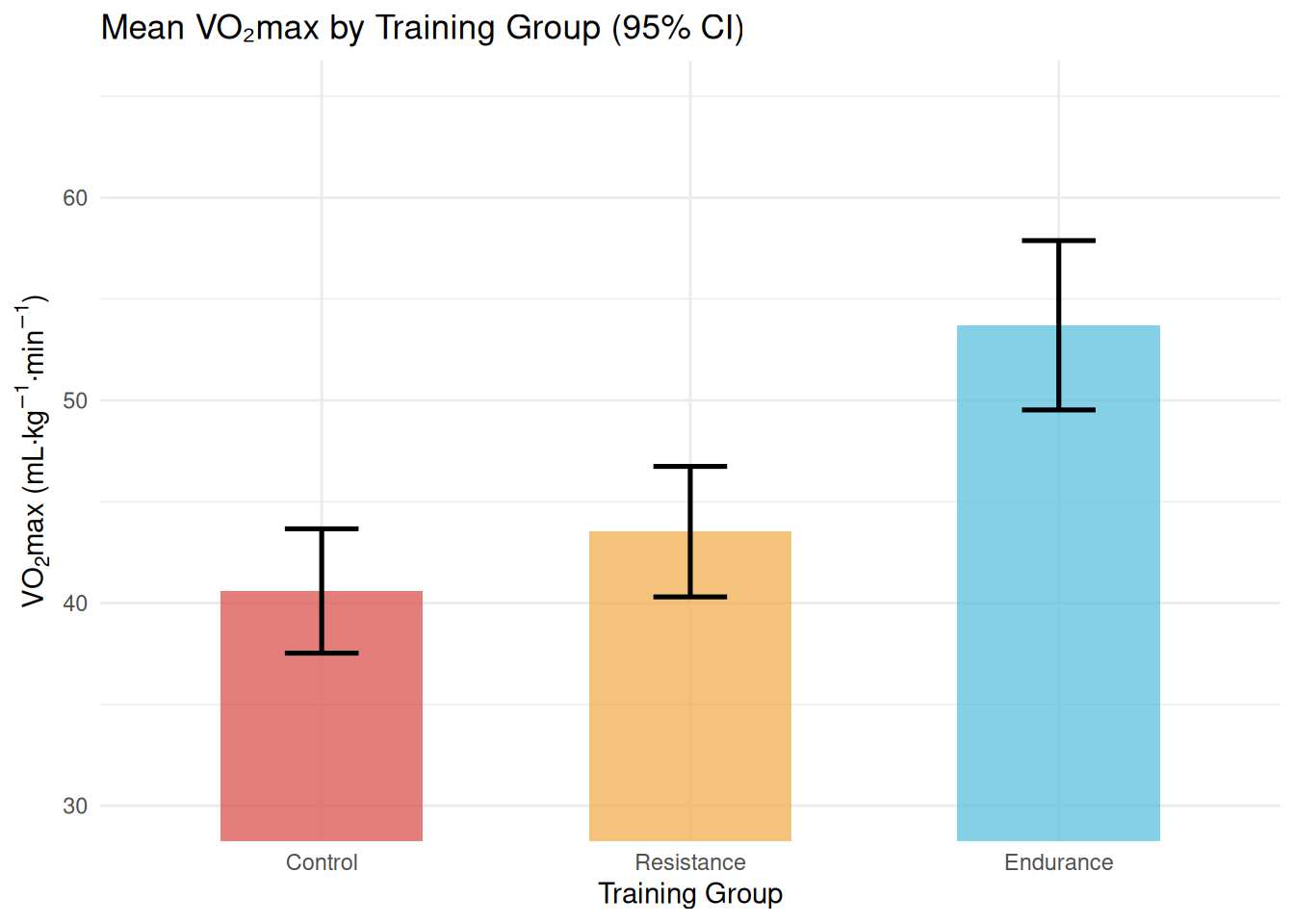
library(ggplot2)library(dplyr)summary_vo2 <- vo2 %>%group_by(Group) %>%summarise(Mean =mean(VO2max),SD =sd(VO2max),n =n(),SE = SD /sqrt(n),CI_lower = Mean -qt(0.975, df = n -1) * SE,CI_upper = Mean +qt(0.975, df = n -1) * SE )ggplot(summary_vo2, aes(x = Group, y = Mean, fill = Group)) +geom_col(alpha =0.75, width =0.55) +geom_errorbar(aes(ymin = CI_lower, ymax = CI_upper),width =0.2, linewidth =0.9) +scale_fill_manual(values =c("Control"="#d9534f","Resistance"="#f0ad4e","Endurance"="#5bc0de")) +labs(x ="Training Group", y =expression(VO[2]*"max (mL·kg"^-1*"·min"^-1*")"),title ="Mean VO₂max by Training Group (95% CI)") +coord_cartesian(ylim =c(30, 65)) +theme_minimal() +theme(legend.position ="none")
Figure 14.2: Mean VO₂max (mL·kg⁻¹·min⁻¹) with 95% confidence intervals for each training group. Non-overlapping confidence intervals between the endurance and control groups strongly suggest a statistically significant difference.
Error bar plots with 95% confidence intervals (Figure 14.2) complement formal testing by conveying both the magnitude and precision of group differences. When CIs do not overlap, this provides a visual indication that the corresponding groups likely differ significantly; however, overlapping CIs do not rule out significance at α = .05, so formal ANOVA and post hoc tests are always necessary[22].
14.10 Reporting ANOVA results in APA style
14.10.1 Omnibus F-test
Template:
“A one-way ANOVA revealed a [significant/non-significant] effect of [factor] on [DV], F([df_B], [df_W]) = [F-value], p = [p-value], η² = [value] (or ω² = [value]).”
Example:
“A one-way ANOVA revealed a significant effect of training group on VO₂max, F(2, 57) = 14.87, p < .001, η² = .34, ω² = .32.”
14.10.2 Post hoc comparisons
Template (following significant omnibus F):
“Post hoc comparisons using [test name] indicated that [Group A] (M = [value], SD = [value]) differed significantly from [Group B] (M = [value], SD = [value]), p = [value], 95% CI [lower, upper].”
Full example:
“A one-way ANOVA revealed a significant effect of training group on VO₂max, F(2, 57) = 14.87, p < .001, η² = .34, ω² = .32. Post hoc comparisons using Tukey HSD indicated that the endurance group (M = 52.4, SD = 6.8 mL·kg⁻¹·min⁻¹) had significantly higher VO₂max than both the resistance group (M = 45.2, SD = 6.2), p = .003, 95% CI [2.1, 12.3], and the control group (M = 40.6, SD = 6.4), p < .001, 95% CI [6.7, 16.9]. Resistance and control groups did not differ significantly, p = .082, 95% CI [−0.5, 9.7].”
TipInclude descriptive statistics for each group
Always report group means and standard deviations alongside the omnibus F-test. These allow readers to assess the direction and practical magnitude of differences, independent of the p-value[23,24].
14.11 Sample size and power for ANOVA
Statistical power in one-way ANOVA depends on the same factors as the t-test: sample size, effect size (Cohen’s f), and α level — plus the number of groups[8,21].
Power analysis for ANOVA is most conveniently performed using G*Power, a free and widely used software package[21]. To conduct a prospective power analysis (determining the sample size needed before collecting data), open G*Power, set the test family to F tests and the statistical test to ANOVA: Fixed effects, omnibus, one-way, then select A priori under the type of power analysis. You will need to specify four values: the expected effect size Cohen’s f (derived from pilot data, prior literature, or the small/medium/large benchmarks of .10, .25, and .40, respectively), the desired α level (typically .05), the target power level (typically .80 or .90), and the number of groups in your design.
Effect size is the most consequential and most difficult of these inputs. Rather than defaulting to a “medium” effect, researchers are encouraged to base their effect size estimate on the smallest effect that would be meaningful or detectable in their specific context — an approach sometimes called the smallest effect size of interest[9]. If pilot data are available, compute Cohen’s f from the observed η² using \(f = \sqrt{\eta^2 / (1 - \eta^2)}\) and use that value as the input. For example, to detect a medium effect (f = .25) with 80% power and α = .05 across three groups, G*Power indicates approximately 52 total participants — about 17 per group — are required[8,21]. Increasing the number of groups while holding effect size and power constant requires proportionally larger samples, since each additional group adds degrees of freedom to the denominator without contributing additional between-group signal.
TipExplore power with the in-book calculator — then confirm with G*Power or SPSS
The Statistical Calculators appendix includes an interactive power calculator that supports one-way ANOVA alongside t-tests and correlations. It is a great way to build intuition: try adjusting the effect size, number of groups, or sample size and watch how power responds in real time. This kind of exploration — rather than just solving for a single required N — is how researchers develop a practical feel for these relationships.
For formal research planning, confirm your estimates with dedicated software. G*Power (free, downloadable at psychologie.hhu.de) has long been the standard for movement science power analyses and is widely cited in published methods sections[21]. SPSS Statistics 31 and later now includes a built-in power analysis module under Analyze → Power Analysis, letting you estimate required sample sizes or post-hoc achieved power without leaving the software you already use for your analyses.
14.12 Common pitfalls and best practices
14.12.1 Pitfall 1: Running multiple t-tests instead of ANOVA
Problem: Conducting separate t-tests for each pair inflates familywise Type I error far beyond α[2].
Solution: Always use ANOVA for the omnibus test across three or more groups, then apply post hoc tests for pairwise comparisons.
14.12.2 Pitfall 2: Running post hoc tests without a significant omnibus F
Problem: Conducting pairwise comparisons after a non-significant F capitalizes on chance and produces unreliable results.
Solution: Post hoc tests are only appropriate following a statistically significant omnibus F-test[4,11].
14.12.3 Pitfall 3: Reporting η² without acknowledging its bias
Problem: η² systematically overestimates the population effect in small samples, presenting a more optimistic picture than warranted.
Solution: Report ω² as the primary effect size, or note η²’s upward bias when reporting it[9,20].
14.12.4 Pitfall 4: Treating a non-significant F as proof of no difference
Problem: Failing to reject H₀ does not establish that group means are equal — it only means the evidence was insufficient to detect a difference, which may reflect low power[25,26].
Solution: Always report effect sizes and confidence intervals. A non-significant result with a wide CI and moderate effect size calls for a larger study, not the conclusion that groups do not differ.
14.12.5 Pitfall 5: Ignoring unequal group sizes
Problem: Highly unbalanced designs (very unequal n per group) reduce power and may affect assumption checks.
Solution: Aim for approximately equal group sizes whenever possible. When designs are unbalanced, use Type III sums of squares and report group-specific descriptive statistics[2,15].
14.13 Chapter summary
Analysis of Variance is the natural extension of the two-group t-test to situations involving three or more group means, and it is among the most widely used statistical procedures in Movement Science research[1,5]. Its primary motivation is the multiple comparisons problem: running separate t-tests for all possible pairs of groups inflates the familywise Type I error rate to unacceptable levels, while ANOVA tests the omnibus null hypothesis in a single, coherent analysis that preserves the stated α[2]. The conceptual core of ANOVA — partitioning total variance into between-groups and within-groups components — provides a remarkably versatile framework that extends to repeated-measures designs (Chapter 15), factorial designs with multiple factors (Chapter 16), and analysis of covariance (Chapter 17).
Interpreting ANOVA results requires looking beyond the omnibus F-test. A significant F indicates that somewhere among the groups a difference exists; post hoc tests (Tukey HSD when variances are equal, Games-Howell when they are not) identify which specific pairs of groups differ, while controlling the familywise error rate[11,16]. Effect sizes quantify how large these differences are in practical terms: η² expresses the proportion of total variance explained by the factor, while ω² provides a less biased estimate that is preferred for small-to-moderate samples[9,20]. Cohen’s f links effect size to power analysis, enabling researchers to determine the sample sizes needed for adequately powered studies[8,21].
Throughout this chapter — as in Chapter 13 — the emphasis has been on integrating hypothesis testing with effect size estimation and practical significance evaluation[19,27]. A significant p-value confirms that a difference is unlikely due to chance; a large η² or ω² confirms it is meaningful in magnitude; and confidence intervals around post hoc mean differences reveal its real-world size and precision. Together, these elements allow Movement Science researchers to answer not just “Did the groups differ?” but “How much did they differ, how precisely do we know, and does it matter for practice?”[6,18].
14.14 Key terms
one-way ANOVA; analysis of variance; familywise error rate; omnibus test; between-groups variance; within-groups variance; sum of squares; mean square; F-ratio; F-distribution; source table; degrees of freedom; homogeneity of variance; Levene’s test; post hoc test; Tukey HSD; Bonferroni correction; Games-Howell; eta-squared; omega-squared; Cohen’s f; effect size; statistical power
14.15 Practice: quick checks
When comparing k groups, every additional pairwise t-test adds another opportunity for a Type I error. The familywise error rate is 1 − (1 − α)^c, where c is the number of comparisons. With three groups (three tests) at α = .05, the familywise rate rises to approximately .14; with five groups (ten tests), it approaches .40[2]. This means that even if there are no real group differences, a researcher has a 40% chance of finding at least one spuriously significant result. ANOVA solves this by evaluating all group means simultaneously in a single test that maintains the stated α level[1,4].
The F-ratio is the ratio of between-groups mean square to within-groups mean square: F = MS_between / MS_within. MS_between reflects how much group means deviate from the grand mean (signal), while MS_within reflects how much individuals vary within their own groups (noise). When the null hypothesis is true — all group means are equal — both MS components estimate the same population variance, and F ≈ 1. F becomes large when group means differ substantially relative to the variability within groups, indicating that between-group variation is unlikely due to sampling error alone[2,3]. In Movement Science, large F-values often arise when comparing groups with clearly distinct training histories or fitness profiles.
The choice depends primarily on whether the homogeneity of variance assumption is met[4]. When Levene’s test is non-significant (variances are approximately equal), Tukey HSD is the standard recommendation — it controls the familywise error rate well while maintaining good power for pairwise comparisons[11]. When Levene’s test is significant (variances are unequal) or group sizes are very unequal, Games-Howell is preferred because it does not assume equal variances and adjusts both the test statistic and degrees of freedom accordingly[16]. The Bonferroni correction is a conservative alternative suitable for any situation, particularly when the number of planned comparisons is small.
Both η² and ω² quantify the proportion of variance in the dependent variable attributable to the factor[20]. Eta-squared (η² = SS_between / SS_total) is straightforward to compute but is a biased estimator of the population effect size — it tends to overestimate, especially in small samples. Omega-squared (ω²) includes a correction term that penalizes for the number of groups and the within-groups variance, making it less biased and more accurate for generalizing to the population[9]. ω² is preferred for reporting, particularly with small samples (total N < 100). Eta-squared remains widely used in published research, so it is worth reporting both and noting η²’s upward bias to aid transparent interpretation.
With p = .083 > α = .05, the omnibus F-test is not significant and the researcher fails to reject H₀. This means the evidence is insufficient to conclude that any group means differ — but it does not prove that the groups are equal[25,26]. The researcher should report the F-statistic, degrees of freedom, and p-value, and also compute and report the effect size (ω²) and its confidence interval. If ω² is modest and the CI is wide, the study may be underpowered; a larger sample size should be considered for future research. Critically, post hoc tests should not be run following a non-significant omnibus result, as doing so inflates Type I error[4].
The three assumptions are: (1) Independence of observations — scores are not influenced by other participants. This must be ensured by design (random, independent sampling); there is no statistical correction for non-independence. (2) Normality — the DV is approximately normally distributed within each group. ANOVA is robust to mild departures from normality with larger samples (n ≥ 30 per group)[12]; severe violations can be addressed with data transformations or the nonparametric Kruskal-Wallis test (Chapter 19)[10]. (3) Homogeneity of variance — population variances are approximately equal across groups, assessed with Levene’s test[14]. When violated, use Welch’s ANOVA or Brown-Forsythe ANOVA with Games-Howell post hoc tests[4,16].
NoteRead further
For deeper exploration of ANOVA and experimental design, see Maxwell, Delaney & Kelley (2018)[2] (Designing Experiments and Analyzing Data), Field (2018)[4] (Discovering Statistics Using IBM SPSS), Cohen (1988)[8] for effect size planning, and Olejnik & Algina (2003)[20] for guidance on unbiased effect size estimation. For Movement Science applications, consult Vincent (2005)[5] and Hopkins et al. (2009)[18].
TipNext chapter
In Chapter 15, you will extend the ANOVA framework to repeated measures designs, in which the same participants are measured across multiple conditions or time points. You will learn about the sphericity assumption, Mauchly’s test, and corrections (Greenhouse-Geisser, Huynh-Feldt), as well as how within-subject designs dramatically increase statistical power by removing between-subject variability from the error term.
1. Fisher, R. A. (1925). Statistical methods for research workers.
2. Maxwell, S. E., Delaney, H. D., & Kelley, K. (2018). Designing experiments and analyzing data: A model comparison perspective (3rd ed.). Routledge.
3. Moore, D. S., McCabe, G. P., & Craig, B. A. (2021). Introduction to the practice of statistics (10th ed.). W. H. Freeman; Company.
4. Field, A. (2018). Discovering statistics using IBM SPSS statistics (5th ed.). SAGE Publications.
5. Vincent, W. J. (2005). Statistics in kinesiology.
7. Portney, L. G., & Watkins, M. P. (2020). Foundations of clinical research: Applications to practice.
8. Cohen, J. (1988). Statistical power analysis for the behavioral sciences (2nd ed.). Lawrence Erlbaum Associates.
9. Lakens, D. (2013). Calculating and reporting effect sizes to facilitate cumulative science: A practical primer for t-tests and ANOVAs. Frontiers in Psychology, 4, 863. https://doi.org/10.3389/fpsyg.2013.00863
10. Conover, W. J. (1999). Practical nonparametric statistics.
11. Tukey, J. W. (1949). Comparing individual means in the analysis of variance. Biometrics, 5(2), 99–114. https://doi.org/10.2307/3001913
12. Blanca, M. J., Alarcón, R., Arnau, J., Bono, R., & Bendayan, R. (2013). Non-normal data: Is ANOVA still a valid option? Psicothema, 25(4), 552–557. https://doi.org/10.7334/psicothema2013.552
13. Lumley, T., Diehr, P., Emerson, S., & Chen, L. (2002). The importance of the normality assumption in large public health data sets. Annual Review of Public Health, 23, 151–169. https://doi.org/10.1146/annurev.publhealth.23.100901.140546
14. Levene, H. (1960). Robust tests for equality of variances. Contributions to Probability and Statistics: Essays in Honor of Harold Hotelling, 278–292.
15. Tabachnick, B. G., & Fidell, L. S. (2019). Using multivariate statistics.
16. Games, P. A., & Howell, J. F. (1976). Pairwise multiple comparison procedures with unequal n’s and/or variances: A monte carlo study. Journal of Educational Statistics, 1(2), 113–125. https://doi.org/10.3102/10769986001002113
18. Hopkins, W. G., Marshall, S. W., Batterham, A. M., & Hanin, J. (2009). Progressive statistics for studies in sports medicine and exercise science. Medicine & Science in Sports & Exercise, 41(1), 3–13. https://doi.org/10.1249/MSS.0b013e31818cb278
20. Olejnik, S., & Algina, J. (2003). Generalized eta and omega squared statistics: Measures of effect size for some common research designs. Psychological Methods, 8(4), 434–447. https://doi.org/10.1037/1082-989X.8.4.434
21. Faul, F., Erdfelder, E., Lang, A.-G., & Buchner, A. (2007). G*power 3: A flexible statistical power analysis program for the social, behavioral, and biomedical sciences. Behavior Research Methods, 39(2), 175–191. https://doi.org/10.3758/BF03193146
22. Cumming, G. (2012). Understanding the new statistics: Effect sizes, confidence intervals, and meta-analysis. Routledge.
23. Wilkinson, L., & Task Force on Statistical Inference. (1999). Statistical methods in psychology journals: Guidelines and explanations. American Psychologist, 54(8), 594–604. https://doi.org/10.1037/0003-066X.54.8.594
24. American Psychological Association. (2020). Publication manual of the american psychological association (7th ed.). American Psychological Association.
26. Altman, D. G., & Bland, J. M. (1995). Statistics notes: Absence of evidence is not evidence of absence. BMJ, 311, 485. https://doi.org/10.1136/bmj.311.7003.485
27. Batterham, A. M., & Hopkins, W. G. (2006). Making meaningful inferences about magnitudes. International Journal of Sports Physiology and Performance, 1(1), 50–57. https://doi.org/10.1123/ijspp.1.1.50