par(mfrow = c(1, 2), mar = c(4, 4, 3, 2))
# Parameters
mu <- 52
se <- 1.1
xbar <- 53 # Observed sample mean (different from μ to show the concept)
ci_multiplier <- 2 # approximately 95%
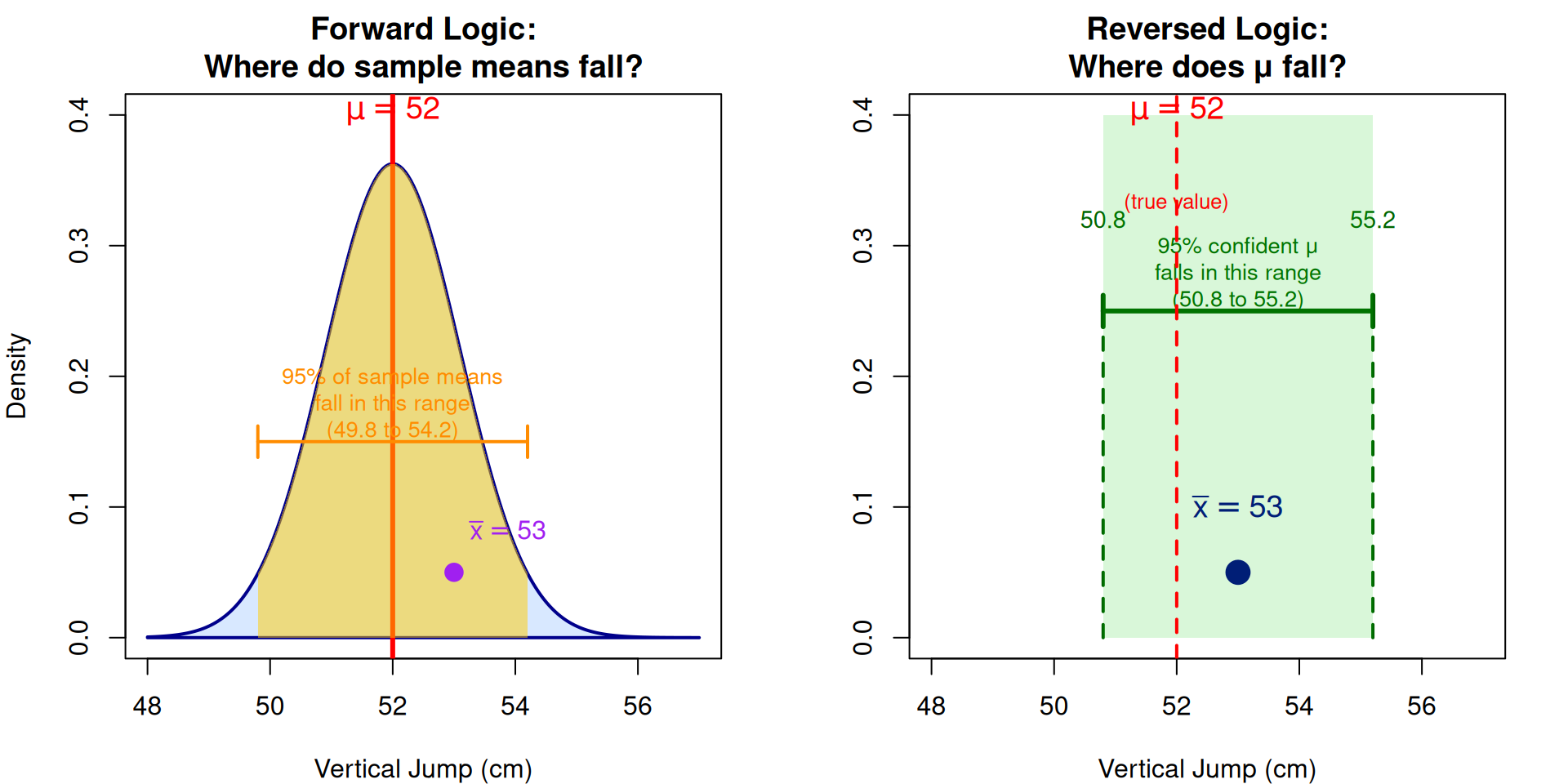
# LEFT PANEL: Forward logic (sampling distribution)
plot(NULL, xlim = c(48, 57), ylim = c(0, 0.4),
xlab = "Vertical Jump (cm)", ylab = "Density",
main = "Forward Logic:\nWhere do sample means fall?")
# Draw sampling distribution centered at μ
x_vals <- seq(48, 57, length.out = 200)
y_vals <- dnorm(x_vals, mean = mu, sd = se)
polygon(c(x_vals, rev(x_vals)), c(y_vals, rep(0, length(y_vals))),
col = rgb(0.5, 0.7, 1, 0.3), border = "darkblue", lwd = 2)
# Mark μ and the 95% interval
abline(v = mu, col = "red", lwd = 3, lty = 1)
text(mu, 0.38, expression(mu == 52), col = "red", cex = 1.2, pos = 3)
# Shade 95% region
x_95 <- seq(mu - ci_multiplier*se, mu + ci_multiplier*se, length.out = 100)
y_95 <- dnorm(x_95, mean = mu, sd = se)
polygon(c(x_95, rev(x_95)), c(y_95, rep(0, length(y_95))),
col = rgb(1, 0.8, 0, 0.5), border = NA)
# Mark boundaries
arrows(mu - ci_multiplier*se, 0.15, mu + ci_multiplier*se, 0.15,
code = 3, angle = 90, length = 0.1, lwd = 2, col = "darkorange")
text(mu, 0.18, "95% of sample means\nfall in this range\n(49.8 to 54.2)", cex = 0.85, col = "darkorange")
# Mark the observed sample mean
points(xbar, 0.05, pch = 19, cex = 1.5, col = "purple")
text(xbar, 0.08, expression(bar(x) == 53), col = "purple", cex = 1, pos = 4)
# RIGHT PANEL: Reversed logic (confidence interval)
plot(NULL, xlim = c(48, 57), ylim = c(0, 0.4),
xlab = "Vertical Jump (cm)", ylab = "",
main = "Reversed Logic:\nWhere does μ fall?")
# Draw a point for observed sample mean
points(xbar, 0.05, pch = 19, cex = 2, col = "darkblue")
text(xbar, 0.08, expression(bar(x) == 53), col = "darkblue", cex = 1.2, pos = 3)
# Draw confidence interval around xbar
arrows(xbar - ci_multiplier*se, 0.25, xbar + ci_multiplier*se, 0.25,
code = 3, angle = 90, length = 0.1, lwd = 3, col = "darkgreen")
text(xbar, 0.28, "95% confident μ\nfalls in this range\n(50.8 to 55.2)", cex = 0.85, col = "darkgreen")
# Mark the interval bounds
segments(xbar - ci_multiplier*se, 0, xbar - ci_multiplier*se, 0.25,
lty = 2, col = "darkgreen", lwd = 2)
segments(xbar + ci_multiplier*se, 0, xbar + ci_multiplier*se, 0.25,
lty = 2, col = "darkgreen", lwd = 2)
text(xbar - ci_multiplier*se, 0.32, "50.8", cex = 0.9, col = "darkgreen")
text(xbar + ci_multiplier*se, 0.32, "55.2", cex = 0.9, col = "darkgreen")
# Add a shaded region to show where μ likely is
rect(xbar - ci_multiplier*se, 0, xbar + ci_multiplier*se, 0.4,
col = rgb(0, 0.8, 0, 0.15), border = NA)
# Mark the true μ to show it falls within the CI
abline(v = mu, col = "red", lwd = 2, lty = 2)
text(mu, 0.38, expression(mu == 52), col = "red", cex = 1.2, pos = 3)
text(mu, 0.35, "(true value)", col = "red", cex = 0.8, pos = 1)
par(mfrow = c(1, 1))