A Note on By-Hand Calculations: The purpose of this book is not to teach tedious by-hand statistical calculations. Modern researchers run these analyses using major software packages. While we provide the underlying equations for conceptual understanding, we strongly recommend relying on software for computation to avoid errors and save time.
Please direct your attention to the SPSS Tutorial: Clinical Measures in the appendix for step-by-step instructions on computing responder rates, sensitivity, specificity, likelihood ratios, and ROC curves in SPSS!
NoteLearning objectives
By the end of this chapter, you will be able to:
Distinguish between statistical significance and clinical meaningfulness, and explain why a significant p-value does not guarantee a clinically important finding.
Define the Minimal Clinically Important Difference (MCID) and apply both distribution-based and anchor-based methods to estimate it.
Calculate and interpret the Number Needed to Treat (NNT), Absolute Risk Reduction (ARR), and Relative Risk (RR).
Construct a 2 × 2 contingency table and compute sensitivity, specificity, positive predictive value (PPV), negative predictive value (NPV), and likelihood ratios.
Interpret ROC curves and the Area Under the Curve (AUC) as a global measure of a diagnostic test’s discriminative ability.
Integrate p-values, effect sizes, MDC, and MCID into a coherent narrative of clinical significance.
20.1 Chapter Roadmap
Every chapter in this textbook has worked toward the same goal: extracting reliable, quantified information from movement science data. By now you can compute t-tests, ANOVA, regression, and reliability coefficients, and you know how to report them correctly. But there is a question that statistical output alone cannot answer:
Does this change actually matter to the patient or athlete in front of me?
A training programme may produce a statistically significant improvement in functional ability — F(1, 57) = 130, p < .001 — but if the mean gain is only 2 points on a 100-point scale, a clinician may reasonably conclude that the intervention offers no meaningful benefit. Conversely, a study with small sample size may produce p = .09 on a 15-point gain that every physiotherapist would consider transformative. The p-value and the clinical verdict do not always align.
This chapter introduces the tools that bridge statistical output and clinical decision-making. The first set of tools — the Minimal Clinically Important Difference (MCID) and the responder approach — ask whether individual patients changed by enough to matter. The second set — Number Needed to Treat (NNT) and related risk statistics — translate group-level effects into statements about how often treatment works. The third set — sensitivity, specificity, likelihood ratios, and ROC analysis — evaluates how accurately a test or measurement identifies the people who need a particular intervention or diagnosis. Together, these tools form the language of clinical evidence.
20.2 Statistical Significance vs. Clinical Meaningfulness
Before introducing formal methods, it is worth examining the tension between statistical and clinical significance directly.
Statistical significance (p < .05) tells you that an observed difference is unlikely to have arisen by chance alone, given the null hypothesis. It is a probability statement about the data, not about the magnitude or importance of the effect.
Clinical meaningfulness asks whether the effect is large enough to matter in practice — to a patient making treatment decisions, to a clinician choosing between interventions, or to a coach designing a programme. This is a judgement about magnitude, not probability.
Three things can drive a wedge between them:
Large samples inflate statistical significance. With N = 2,000, a 0.5-point improvement on a 100-point scale will almost certainly be statistically significant (p < .001), yet no clinician would consider half a point a meaningful recovery. The larger the sample, the more easily small, inconsequential differences achieve significance.
Small samples suppress it. A 15-point improvement in a pilot study of 8 participants may fail to reach p < .05 simply because the study is underpowered, even though the effect is clinically important.
Effect sizes help but do not fully solve the problem. Cohen’s d = 0.40 is “small-to-medium” by convention, but that benchmark was calibrated against social-science data, not physiotherapy outcomes. A d of 0.40 on a pain scale might represent a change that patients notice every day; the same d on a laboratory VO₂max test might be clinically trivial.
The solution is to supplement p-values and effect sizes with measures that are calibrated against patients’ actual experience — the MCID, NNT, and diagnostic accuracy statistics introduced in this chapter[1,2].
NoteThe “so what?” test
A practical habit when reviewing statistical results is to ask: “So what does this mean for the person I’m treating?” If the answer is “very little,” report the finding honestly and acknowledge the gap between statistical and clinical significance. Overstating the clinical relevance of statistically significant but small effects is one of the most common sources of misleading conclusions in movement science research.
20.3 The Responder Approach
Rather than asking whether the group mean changed significantly, the responder approach asks: “What proportion of individuals changed enough to be classified as improved?” This reframes the analysis from a group-average question to a person-level question — which is often what clinicians and patients actually care about.
A responder is a participant whose change score meets or exceeds a pre-defined threshold. That threshold is usually the MCID (defined in the next section), the MDC₉₅ (Chapter 18), or a clinically established cut-point.
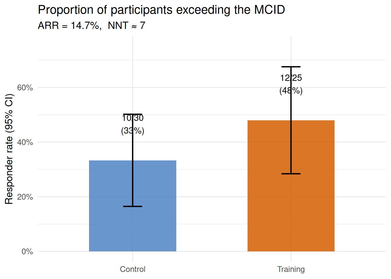
Example. In the training group (n = 25 with complete pre/post data), 12 participants improved their functional ability (function_0_100) by at least 6.1 points — the MCID for this measure. That is a responder rate of 48%. In the control group (n = 30), 10 participants improved by the same threshold without any intervention — a spontaneous responder rate of 33%. The training programme elevated the responder rate by 15 percentage points.
This simple comparison immediately conveys something a mean difference cannot: the training programme helped roughly half of participants meaningfully, but not everyone. A clinician reading only the significant group-mean ANCOVA from Chapter 17 might assume the programme works for everyone; the responder analysis corrects that impression.
TipChoosing the right threshold
The responder threshold should be established before data collection, ideally based on published MCID estimates for the outcome measure, patient-reported anchor data, or the MDC₉₅ from a separate reliability study. Post-hoc selection of convenient thresholds that maximise the responder rate is a form of selective reporting and inflates the apparent benefit of an intervention.
20.4 Minimal Clinically Important Difference (MCID)
The Minimal Clinically Important Difference is the smallest change in an outcome that a patient (or clinician) would perceive as meaningful[1]. It is the threshold below which a change, even if real and statistically significant, is too small to matter in practice.
MCID differs from MDC₉₅ (Chapter 18) in an important way:
MDC₉₅ is a measurement property — the smallest change that exceeds measurement error at the 95% confidence level. A change below MDC₉₅ may simply be noise.
MCID is a clinical property — the smallest change that patients experience as worthwhile. MCID may be larger or smaller than MDC₉₅ depending on the measure and the population.
For clinical interpretation, both thresholds matter. A change that exceeds MDC₉₅ but falls below MCID is real (it is not measurement error) but clinically unimportant. A change that exceeds MCID but falls below MDC₉₅ is clinically desired but statistically indistinguishable from noise. The ideal scenario is a change that exceeds both.
20.4.1 Methods for estimating MCID
Two broad approaches are used:
Distribution-based methods anchor the MCID to statistical properties of the outcome measure — its variability, reliability, or measurement error. The most common is the half standard deviation rule: MCID ≈ 0.5 × SD_pre[3]. This rule has been validated across dozens of patient-reported outcomes and consistently approximates the threshold patients describe as “a noticeable difference.” Other distribution-based estimates include 1 SEM (approximately equal to the half-SD rule when reliability is moderate) or effect size Cohen’s d = 0.50.
\[\text{MCID}_{dist} = 0.5 \times SD_{baseline}\]
Anchor-based methods use an external criterion — a global rating of change scale, a transition question (“Is your condition much better, a little better, the same, a little worse, or much worse?”), or a clinical expert’s judgement — to identify what magnitude of change corresponds to a “little better” response[1]. Participants are split by their anchor rating and the mean score change in the “little better” group is taken as the MCID. Anchor-based methods are considered the gold standard because they are directly grounded in patient experience, but they require the collection of anchor data alongside the outcome measure.
Worked example. Using the distribution-based method on the core_session dataset:
Pre-test mean functional ability (full sample): M = 70.2, SD = 12.2 points
MCID = 0.5 × 12.2 = 6.1 points
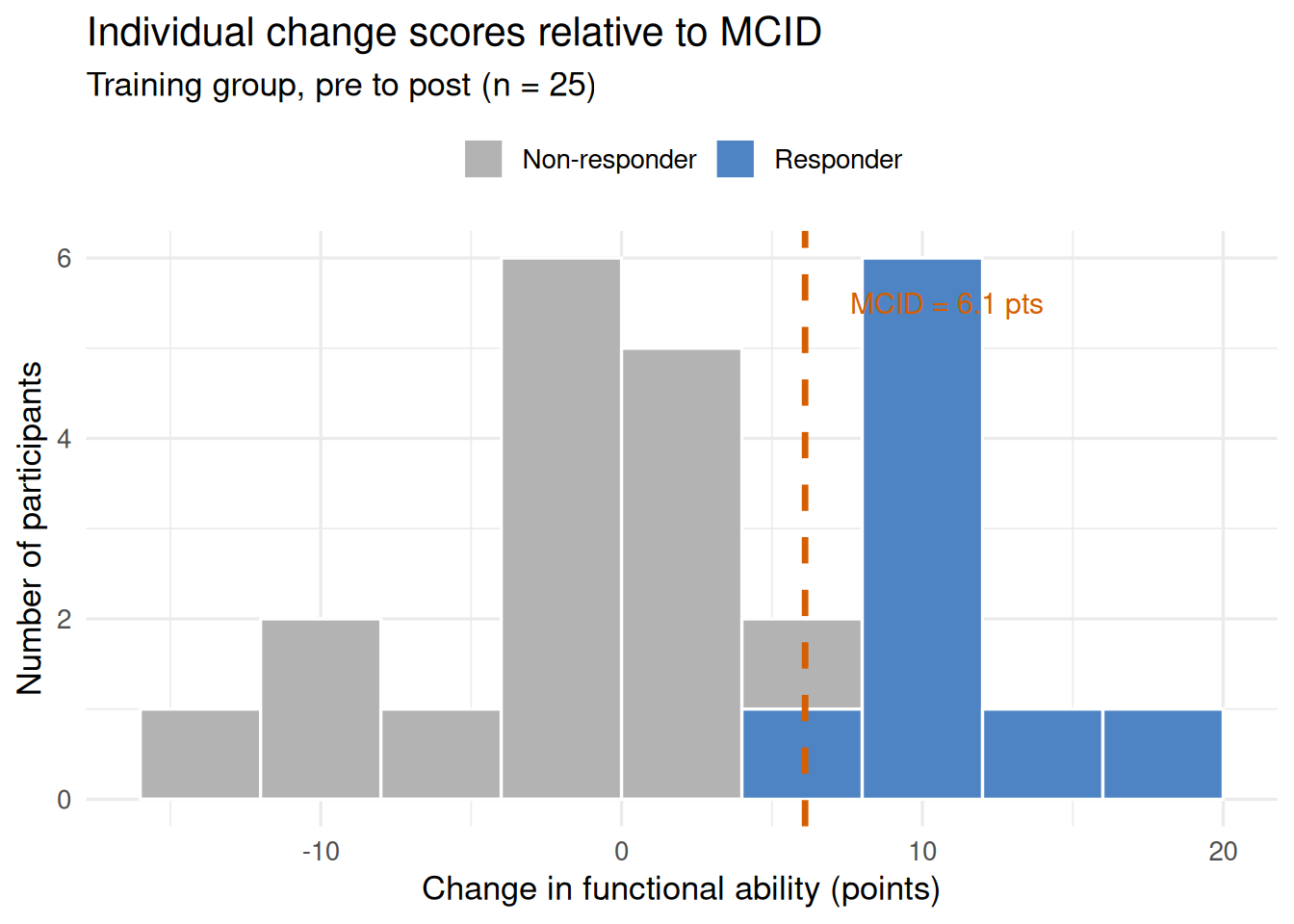
This means a participant must improve by at least 6.1 points on the function_0_100 scale to be classified as a responder — someone who has experienced a meaningful recovery.
Code
set.seed(42)n_tr <-25pre_func <-rnorm(n_tr, 69.5, 14.7)post_func <- pre_func +rnorm(n_tr, 5.0, 8.5)pre_func <-pmin(pmax(pre_func, 0), 100)post_func <-pmin(pmax(post_func, 0), 100)changes <- post_func - pre_funcmcid_val <-6.1df_mcid <-data.frame(change = changes,responder =ifelse(changes >= mcid_val, "Responder", "Non-responder"))ggplot(df_mcid, aes(x = change, fill = responder)) +geom_histogram(binwidth =4, color ="white", boundary =0) +geom_vline(xintercept = mcid_val, linetype ="dashed",color ="#D55E00", linewidth =1.2) +annotate("text", x = mcid_val +1.5, y =5.5,label =paste0("MCID = ", mcid_val, " pts"),hjust =0, color ="#D55E00", size =4) +scale_fill_manual(values =c("Responder"="#4E84C4","Non-responder"="grey70")) +labs(x ="Change in functional ability (points)",y ="Number of participants",fill =NULL,title ="Individual change scores relative to MCID",subtitle ="Training group, pre to post (n = 25)" ) +theme_minimal(base_size =13) +theme(legend.position ="top")
Figure 20.1: Distribution of individual pre-to-post changes in functional ability for the training group (n = 25). The dashed vertical line marks the MCID of 6.1 points (0.5 × SD at baseline). Bars to the right of the line represent responders — participants whose change exceeded the MCID. Twelve of 25 participants (48%) were classified as responders.
WarningMCID is population- and measure-specific
An MCID estimated for one instrument in one population cannot be automatically transferred to a different outcome measure or a different clinical group. The MCID for functional ability in older adults recovering from hip surgery will differ from the MCID for functional ability in young athletes following an ACL reconstruction. Always cite the source of your MCID estimate and verify that it was derived from a population similar to your own.
20.5 Number Needed to Treat (NNT)
The Number Needed to Treat (NNT) is perhaps the most clinically intuitive statistic in evidence-based practice. It answers: “On average, how many patients need to receive this intervention for one additional patient to benefit — beyond what would have occurred without treatment?”[2]
NNT is derived from two quantities:
Experimental Event Rate (EER): the proportion of patients in the treatment group who achieve the desired outcome (e.g., exceed the MCID).
Control Event Rate (CER): the corresponding proportion in the control group.
\[ARR = EER - CER\]
\[NNT = \frac{1}{ARR}\]
where ARR is the Absolute Risk Reduction — the absolute difference in event rates between groups. A lower NNT means a more effective treatment; NNT = 1 would mean every treated patient benefits who would not have benefited otherwise (impossible in practice); NNT = ∞ means treatment adds no benefit over control.
Worked example. Using functional improvement ≥ MCID as the outcome event:
Responders
Total
Event Rate
Training
12
25
EER = .480 (48%)
Control
10
30
CER = .333 (33%)
\[ARR = .480 - .333 = .147 \approx 14.7\%\]
\[NNT = \frac{1}{.147} = 6.8 \approx 7\]
Interpretation. On average, approximately 7 participants need to complete the 12-week training programme for one additional person to achieve a clinically meaningful improvement in functional ability — beyond the spontaneous recovery seen in the control group. This is a concrete, actionable number that clinicians and programme directors can weigh against the cost and burden of the intervention.
Relative Risk (RR) and Relative Risk Reduction (RRR) complement NNT:
The training programme produced a 44% relative increase in the responder rate compared with the control condition. While the RRR appears more impressive than the ARR (44% vs. 15%), the ARR and NNT are more informative because they account for the baseline event rate. An intervention that doubles a 1% event rate (RRR = 100%, ARR = 1%, NNT = 100) is far less impressive than one that doubles a 40% event rate (RRR = 100%, ARR = 40%, NNT = 2.5).
Figure 20.2: Responder rates for the training and control groups. A responder is defined as a participant whose functional ability improved by at least 6.1 points (the MCID). The training group’s responder rate (48%) exceeded the control group’s rate (33%), yielding ARR = 14.7% and NNT ≈ 7.
NoteConfidence interval for NNT
Because NNT is derived from ARR, its uncertainty should also be reported. The 95% CI for NNT is obtained by computing the 95% CI for ARR and then taking the reciprocals of both limits:
If the CI for ARR spans zero (i.e., includes the possibility that EER ≤ CER), the CI for NNT will span infinity and include negative values (i.e., Number Needed to Harm). This signals that the trial was inconclusive about the direction of the treatment effect.
20.6 Sensitivity, Specificity, PPV, and NPV
The statistics in the previous sections describe how well an intervention works at the group level. The statistics in this section describe how well a test — a physical measure, a screening tool, a clinical criterion — works at the individual level to classify people correctly.
These statistics arise whenever a continuous or categorical measurement is used to make a binary decision: does this person have the condition or not? Will this athlete respond to the intervention or not? Should this patient be referred for further investigation?
20.6.1 The 2 × 2 contingency table
All four statistics derive from a single table that cross-classifies test result (positive/negative) against true condition (present/absent):
Condition present
Condition absent
Test positive
True Positive (TP)
False Positive (FP)
Test negative
False Negative (FN)
True Negative (TN)
Sensitivity is the probability that the test correctly identifies people who have the condition:
\[\text{Sensitivity} = \frac{TP}{TP + FN}\]
Specificity is the probability that the test correctly identifies people who do not have the condition:
\[\text{Specificity} = \frac{TN}{TN + FP}\]
Positive Predictive Value (PPV) is the probability that a positive test result reflects the true condition — the proportion of test-positives who actually have the condition:
\[PPV = \frac{TP}{TP + FP}\]
Negative Predictive Value (NPV) is the probability that a negative test result is truly negative — the proportion of test-negatives who truly lack the condition:
\[NPV = \frac{TN}{TN + FN}\]
TipA memory aid
Think of sensitivity and specificity as properties of the test (they do not depend on how common the condition is in the population). Think of PPV and NPV as properties of the result in context (they depend strongly on prevalence). A test can have perfect sensitivity and specificity in a laboratory and yet produce mostly false positives in clinical practice if the condition is rare.
20.6.2 Worked example
Using post-test muscular strength (strength_kg ≥ 79.8 kg, the sample median) as a simple classifier to identify whether a participant was in the training group (condition present = training group):
A post-test strength score above the sample median correctly identifies a training-group participant 66.7% of the time and correctly clears a control-group participant 66.7% of the time. These are modest but above-chance values, consistent with the group overlap seen in the strength data.
20.7 Likelihood Ratios
Likelihood ratios (LRs) are more useful than sensitivity and specificity alone for clinical decision-making because they express how much a test result changes the probability that someone has the condition. They come in two forms:
A +LR of 2.00 means a positive test result (strength ≥ median) makes it twice as likely that the participant was in the training group. A −LR of 0.50 means a negative test result halves the probability. Both values fall in the “small change” range, confirming that while post-test strength carries some group-discriminating information, it is far from a definitive classifier. This is expected: both groups trained under the same conditions except for the resistance programme, and there was natural overlap in pre-test strength.
Using LRs with pre-test probability (Bayes’ theorem). LRs are most powerful when combined with the pre-test probability of a condition (its prevalence in the tested population) using the likelihood ratio nomogram or Bayes’ rule. In a clinical setting with 50% prevalence (equal training and control numbers), a +LR of 2.00 raises the post-test probability from .50 to .67 — useful but not definitive.
20.8 ROC Curves and Area Under the Curve (AUC)
Sensitivity and specificity depend on the cut-point chosen to dichotomise the continuous test score. A Receiver Operating Characteristic (ROC) curve shows how sensitivity and specificity trade off across all possible cut-points simultaneously[5].
How it is constructed. For each possible threshold value of the continuous test:
Plot sensitivity on the y-axis against (1 − specificity) on the x-axis.
Connect the points to form the ROC curve.
A test with no discriminative ability produces a diagonal line from (0, 0) to (1, 1) — for every gain in sensitivity, an equal loss in specificity occurs. A perfect test produces a curve that passes through the top-left corner (sensitivity = 1, 1 − specificity = 0), indicating that a single threshold perfectly separates conditions.
20.8.1 Area Under the Curve (AUC)
The AUC (also written c-statistic) summarises the entire ROC curve in a single number ranging from 0.5 (no discrimination — equivalent to coin-flipping) to 1.0 (perfect discrimination). Conceptually, AUC is the probability that a randomly selected positive case will receive a higher test score than a randomly selected negative case.
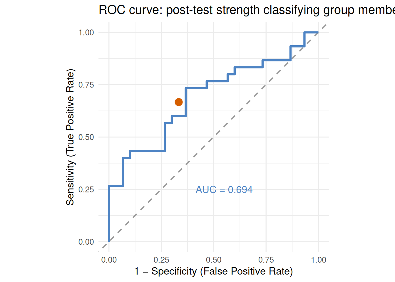
Figure 20.3: ROC curve for post-test strength (strength_kg) as a classifier of group membership (training vs. control), N = 60. The dashed diagonal represents chance performance (AUC = 0.50). The solid curve for post-test strength achieves AUC = .683 (p = .008), indicating acceptable but modest discrimination. The filled point marks the median cut-point (79.8 kg), which yields sensitivity = specificity = .667.
An AUC of .683 falls in the “acceptable” range — post-test strength carries real information about group membership, but alone it is not a reliable classifier. This makes sense: pre-test strength was similar between groups (no selection bias), and not all training-group participants improved by the same amount.
APA write-up:
ROC analysis was conducted to evaluate the ability of post-test muscular strength to discriminate between training and control group participants (N = 60). The AUC was .683 (95% CI [.55, .81]), p = .008, indicating acceptable but modest discrimination. At the optimal cut-point of 79.8 kg, sensitivity was .667 and specificity was .667, with a +LR of 2.00 and −LR of 0.50.
20.9 Linking Statistical and Clinical Significance
With all the tools now assembled, it is possible to construct an integrated picture of the training programme’s effectiveness that moves from statistical inference to clinical reality. Table 20.1 shows how the same dataset speaks differently depending on the type of evidence examined.
Table 20.1: Integrated summary of statistical and clinical evidence for the training programme.
Type of evidence
Finding
What it tells us
ANCOVA p-value
p < .001
The group difference is unlikely due to chance
Effect size (η²_p)
.695 (large)
Most variance in post-strength is accounted for by group × pre-test
MDC₉₅ (Chapter 18)
2.26 kg
Changes > 2.26 kg exceed measurement error
MCID (function)
6.1 points
Changes > 6.1 points are clinically meaningful
Responder rate
48% vs. 33%
About half of trained participants benefited meaningfully
NNT
≈ 7
7 people need to train for 1 additional responder beyond control
AUC (strength)
.683
Post-test strength is a modest group classifier
The key insight from this table is that no single number tells the whole story. The p-value establishes that something real happened. The effect size tells us it was large at the group level. The MDC₉₅ confirms that the change was not just measurement noise. The MCID and responder rate reveal that it was clinically meaningful for about half the participants. The NNT translates this into an actionable dosage for clinical planning. And the AUC shows that post-test strength, while informative, cannot reliably identify who benefited without additional data.
A complete clinical interpretation of any intervention study should address all of these layers, not just the p-value.
20.10 Common Pitfalls
Reporting only p-values without MCID or NNT. A significant p tells readers that a difference exists; it does not tell them whether it matters. Always accompany p-values with at least one measure of clinical meaningfulness — MCID-based responder rates, NNT, or absolute risk differences.
Confusing sensitivity and PPV. A test with 90% sensitivity does not mean 90% of positive results are correct — that is PPV, and it depends on prevalence. In a low-prevalence population, even a highly sensitive test can produce many false positives. Always report PPV and NPV alongside sensitivity and specificity, and note the prevalence on which they were calculated.
Selecting MCID thresholds after observing the data. If the MCID is chosen post-hoc to maximise the responder rate, the analysis is biased. MCID values should come from published literature, external anchor studies, or pre-registered analysis plans.
Over-interpreting AUC. An AUC of .70 may be statistically significant in a large sample but clinically insufficient for screening purposes. In high-stakes decisions (e.g., return-to-sport clearance), AUC values below .85–.90 are generally considered inadequate for stand-alone use. AUC should always be reported with a confidence interval.
Ignoring the confidence interval for NNT. Point estimates of NNT are less informative than NNT with its 95% CI. A NNT of 7 with a CI of [4, 28] conveys that the intervention might be very efficient (1 in 4) or marginally efficient (1 in 28) — a wide range with very different resource implications.
Applying population-level MCID to individuals. The MCID is the average threshold across a group; some individuals may experience meaningful benefit at smaller changes, others only at larger changes. Treat MCID as an approximation, not a precise individual threshold.
20.11 Chapter Summary
Statistical significance is the entry point to interpreting research findings, not the endpoint. This chapter introduced the tools that move beyond the p-value to answer the clinician’s question: does this change matter?
The MCID — estimated as 0.5 × SD_pre or through anchor-based methods — defines the threshold of meaningful change for individual patients. The responder approach classifies individuals against this threshold, revealing what proportion genuinely benefited. NNT translates group-level responder rates into a concrete dosage estimate: approximately 7 participants needed to train for one additional functional responder. Sensitivity, specificity, PPV, NPV, and likelihood ratios evaluate how well a measurement or test classifies individuals, with +LR = 2.00 indicating modest but real discriminative ability for post-test strength. The ROC curve and AUC (.683) summarise this discrimination across all possible cut-points.
Together, these tools form an integrated approach to clinical evidence: statistical inference establishes that effects are real; clinical metrics establish that they matter.
20.11.1 Key terms
Absolute Risk Reduction (ARR) — The difference in event rates between the treatment and control groups; the denominator of NNT.
Area Under the Curve (AUC) — A single summary statistic for the ROC curve representing the probability that a randomly selected positive case scores higher than a randomly selected negative case.
Likelihood ratio — A ratio expressing how much more (or less) likely a test result is among people with the condition than among people without it.
Minimal Clinically Important Difference (MCID) — The smallest change in an outcome that patients or clinicians consider meaningful, estimated via distribution-based or anchor-based methods.
Negative Predictive Value (NPV) — The proportion of negative test results that are true negatives.
Number Needed to Treat (NNT) — The number of patients who must receive an intervention for one additional patient to achieve the desired outcome beyond the control condition.
Positive Predictive Value (PPV) — The proportion of positive test results that are true positives.
Receiver Operating Characteristic (ROC) curve — A graphical display of the trade-off between sensitivity and specificity across all possible test cut-points.
Relative Risk (RR) — The ratio of event rates in the treatment and control groups.
Responder — A participant whose change score meets or exceeds a pre-specified threshold (typically the MCID or MDC₉₅).
Sensitivity — The probability that a test correctly identifies those with the condition (true positive rate).
Specificity — The probability that a test correctly identifies those without the condition (true negative rate).
20.12 Practice: quick checks
The distribution-based MCID = 0.5 × 18.0 = 9.0 points. The observed mean change of 8.2 points falls below the estimated MCID, meaning the statistically significant result does not meet the threshold for clinical meaningfulness. The result is real (it exceeds measurement noise) but smaller than what patients typically perceive as a worthwhile improvement. The colleague’s claim is not supported. A more complete interpretation would note the significant p-value, report the effect size, compare the mean change to both MDC₉₅ and MCID, and examine responder rates at the individual level.
EER = 18/40 = .450; CER = 8/40 = .200. ARR = .450 − .200 = .250 (25%). NNT = 1/.250 = 4.0. RR = .450/.200 = 2.25. The treatment group was 2.25× more likely to respond than controls, with an absolute advantage of 25 percentage points — meaning 4 participants need to be treated for one additional responder beyond spontaneous recovery.
Using a 2 × 2 table for 100 hypothetical athletes (30 truly ready, 70 not ready): TP = 0.80 × 30 = 24; FN = 6. TN = 0.70 × 70 = 49; FP = 21. PPV = 24/45 = .533. NPV = 49/55 = .891. A positive result means only a 53% chance the athlete is truly ready — barely better than a coin flip in this population. The NPV of 89% means a negative result provides reasonable assurance that the athlete is not yet ready. At 30% prevalence, positive results are not sufficiently trustworthy on their own; additional assessment is needed before clearing athletes for return to sport.
An AUC of .62 falls in the “poor” range (0.60–0.70), indicating the test discriminates only slightly better than chance. Although p = .041 is statistically significant, the discrimination is clinically insufficient for most decision-making purposes. Additional information to request: (1) the 95% CI for AUC — if wide (e.g., .51 to .73), the estimate is imprecise; (2) sensitivity and specificity at the optimal cut-point; (3) the prevalence in the clinical population of interest to compute PPV/NPV; (4) the clinical consequences of false positives vs. false negatives, which determine whether higher sensitivity or specificity should be prioritised.
NNT = 1/ARR, and ARR = EER − CER. Several factors cause NNT to differ between studies: (1) Different CERs — if one study’s control group recovers spontaneously at a higher rate, the ARR shrinks and NNT grows. (2) Different MCID thresholds — different cut-points to define “responder” produce different event rates. (3) Different populations — a more severely affected population may show greater treatment response, reducing NNT. (4) Different follow-up periods — longer follow-up allows more control-group participants to recover, raising CER. (5) Sampling variability — with small samples, event rate estimates can vary substantially. NNT should always be reported with a confidence interval and interpreted in the context of the specific study design and population.
The p < .001 establishes that something real happened — the group difference is unlikely to be a chance finding. But it does not tell you how large that difference is, whether individual athletes noticed it, or how many need to train for one to benefit meaningfully. The MCID answers “did individual athletes change enough to feel a difference?” — only 48% of the training group exceeded the MCID, so the impressive group average masks that roughly half did not achieve a meaningful personal improvement. The NNT answers “how efficient is this programme?” — NNT ≈ 7 means 7 athletes must complete the programme for one additional meaningful responder beyond what a control condition would produce. These numbers help the coach decide whether the programme justifies the investment and where modifications might help non-responders. Statistical significance alone cannot answer those questions.
NoteRead further
[1] is the foundational paper on anchor-based MCID methodology.[3] provides the empirical basis for the 0.5 × SD distribution-based rule.[2] is the standard reference for NNT and ARR.[5] offers a comprehensive introduction to ROC analysis and AUC.[4] covers all of these clinical measures within a broader rehabilitation research framework and is the recommended companion text for this chapter.
NoteEnd of Part VI
This chapter completes Part VI: Reliability, Nonparametric Methods, and Clinical Interpretation. Together, Chapters 18–20 equip you to evaluate the precision of your measurements, choose appropriate analyses when parametric assumptions cannot be met, and translate statistical results into clinically meaningful conclusions — the essential final step in evidence-based movement science practice.
1. Jaeschke, R., Singer, J., & Guyatt, G. H. (1989). Measurement of health status: Ascertaining the minimal clinically important difference. Controlled Clinical Trials, 10(4), 407–415. https://doi.org/10.1016/0197-2456(89)90005-6
2. Cook, R. J., & Sackett, D. L. (1995). The number needed to treat: A clinically useful measure of treatment effect. BMJ, 310(6977), 452–454. https://doi.org/10.1136/bmj.310.6977.452
3. Norman, G. R., Sloan, J. A., & Wyrwich, K. W. (2003). Interpretation of changes in health-related quality of life: The remarkable universality of half a standard deviation. Medical Care, 41(5), 582–592. https://doi.org/10.1097/01.MLR.0000062554.74615.4C
4. Portney, L. G., & Watkins, M. P. (2020). Foundations of clinical research: Applications to practice.