Appendix H — Getting Started with SPSS

Installation, Interface, and Basic Workflows

H.1 Purpose & Outcomes

This chapter orients you to SPSS 31 fundamentals. By the end, you will be able to navigate the SPSS interface including the Data Editor, Variable View, Output Viewer, and Syntax Editor. You will learn to set up organized project folders and create reproducible workflows. The chapter covers how to import and enter data with proper metadata, perform basic transformations such as computing new variables and recoding values, and build and export professional charts. You will also learn to run and annotate syntax scripts, conduct essential data integrity checks, and export APA-ready tables and figures for your assignments and research papers.

H.2 Why This Matters

This chapter establishes foundational practices for data management and reproducibility that form the backbone of professional statistical work. The habits you develop here—organizing files systematically, documenting your work, maintaining clean data, and creating reproducible workflows—will serve you throughout your academic career and beyond, regardless of your field or the scale of your projects.

H.2.1 Platforms

SPSS 31 is available for both Windows and macOS. When installing on Windows, run the installer executable and follow the installation wizard, ensuring you have administrator privileges if required. On macOS, follow the standard installation steps and confirm that your system architecture is compatible (Intel or Apple Silicon). On first launch, regardless of platform, you may need to grant necessary permissions for the application to access your files. The license verification screen will appear on the splash screen when you open SPSS for the first time.

SPSS uses either a site license (common for universities) or an individual authorization code. You’ll configure the license manager during initial setup. Be aware of offline grace periods if you need to work without internet access, and understand the renewal process for your institution’s license.

H.2.2 Updates & Folders

You can check for software patches and updates by going to Help > Check for Updates in the menu bar. SPSS stores default user files in locations like Documents/SPSS or similar folders on your system. Understanding where templates and output files are saved will help you locate your work quickly.

H.3 Project Organization

Good file organization is fundamental to successful data analysis. Start by creating a dedicated project folder where you can store all your work in one place. Within this main folder, create subfolders to organize your materials logically: one for raw data files, one for syntax scripts, one for output files, and one for figures and results. This structure makes it easy to locate files months later and simplifies sharing your work with collaborators. Use descriptive file names that clearly indicate content and version—for example, analysis_main.sps for your primary syntax file or results_v02_final.spv for saved output. Include dates in filenames when tracking iterations: data_cleaned_20250110.sav. Establish a consistent naming convention and stick to it throughout your project. Finally, save your work frequently to prevent data loss from unexpected software crashes or computer failures.

H.4 SPSS Interface Tour

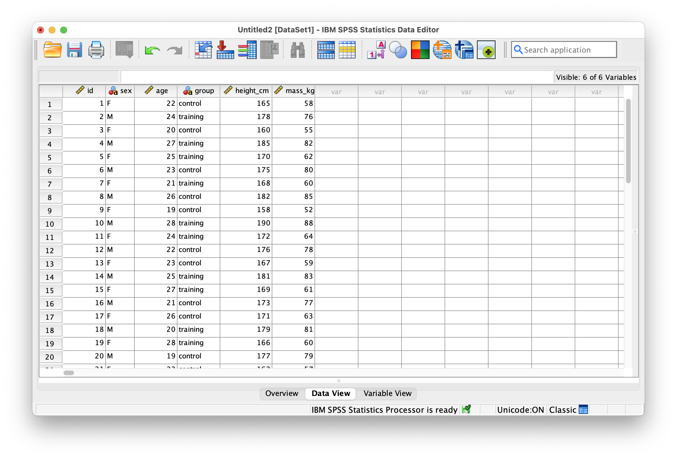
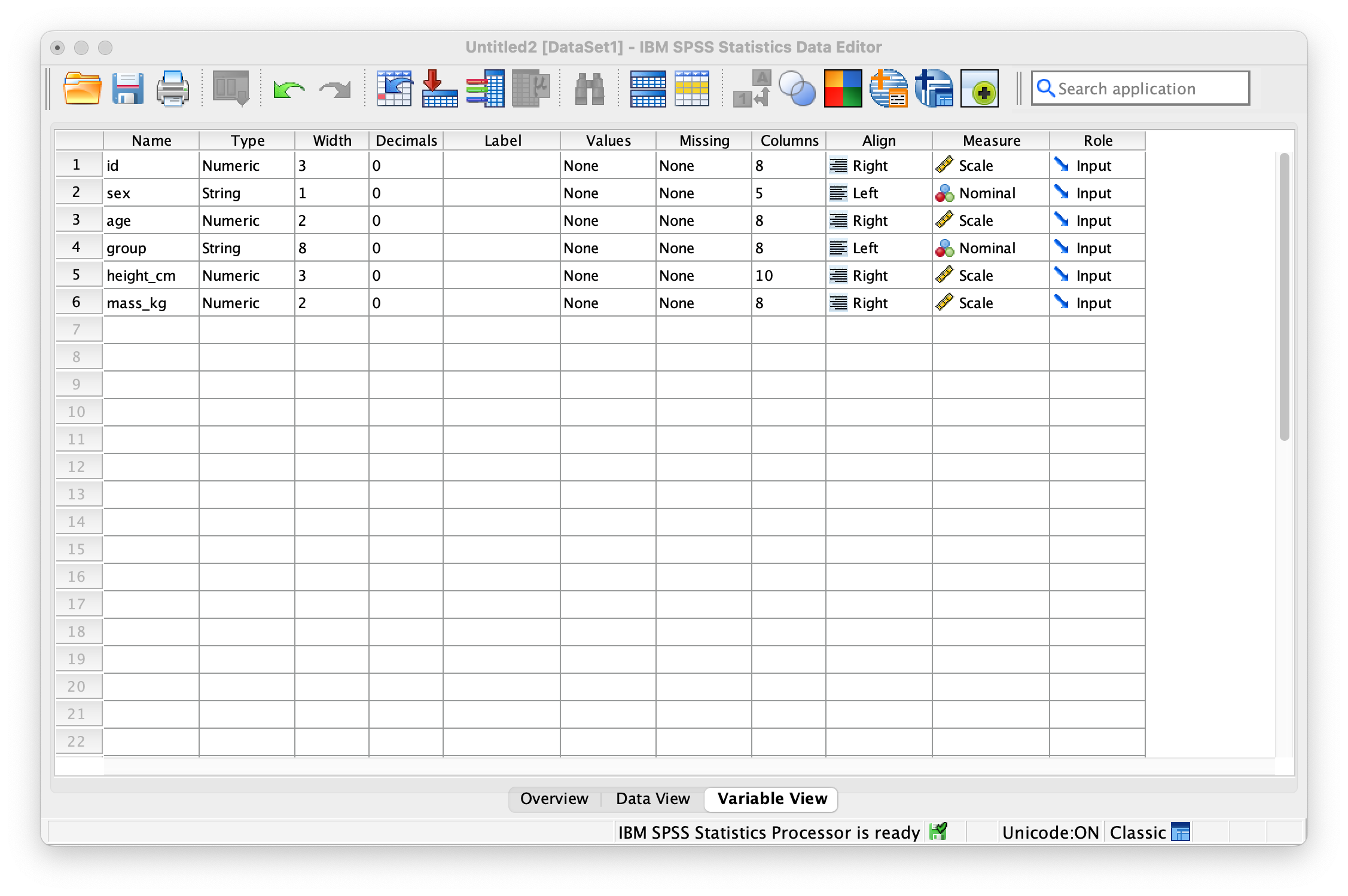
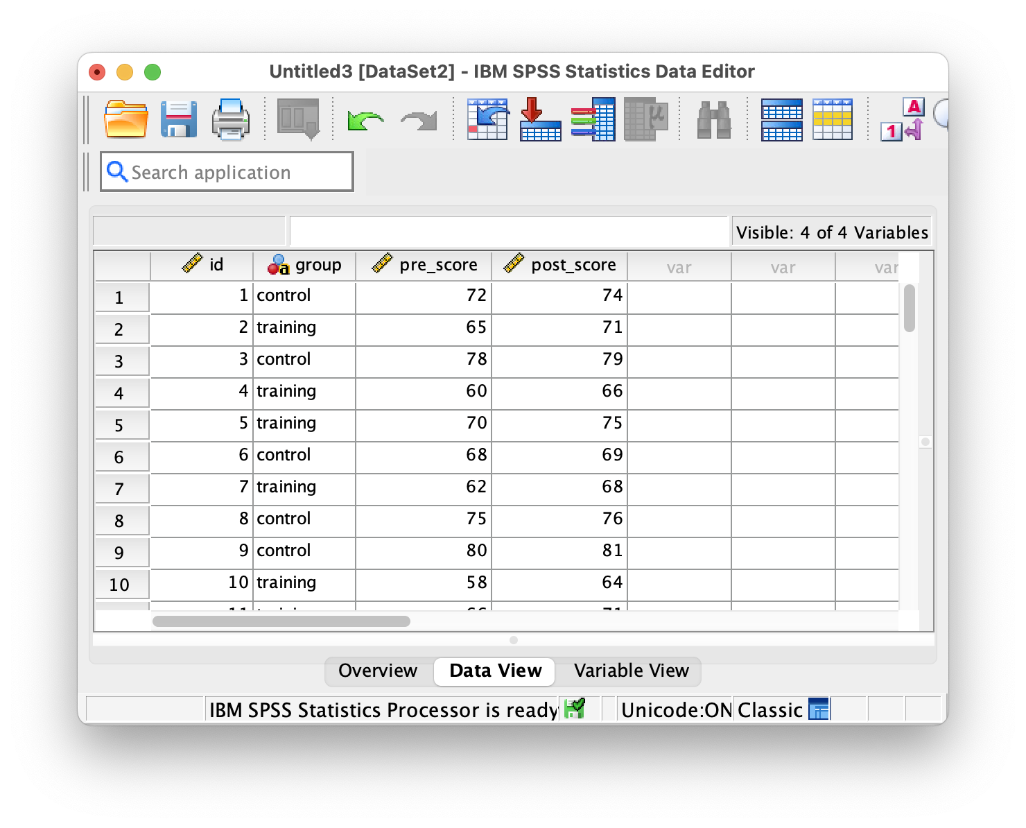
The Data Editor has two main views that you’ll switch between frequently. Data View shows your actual data arranged in rows and columns, where each row represents a case (like a participant) and each column represents a variable (like age or test score). Variable View displays the metadata for each variable, allowing you to define properties like variable type, labels, and missing values.

Figure H.1: Data View

Figure H.2: Variable View

Figure H.3: Output Viewer

Figure H.4: Syntax Editor

H.4.1 Chart Builder

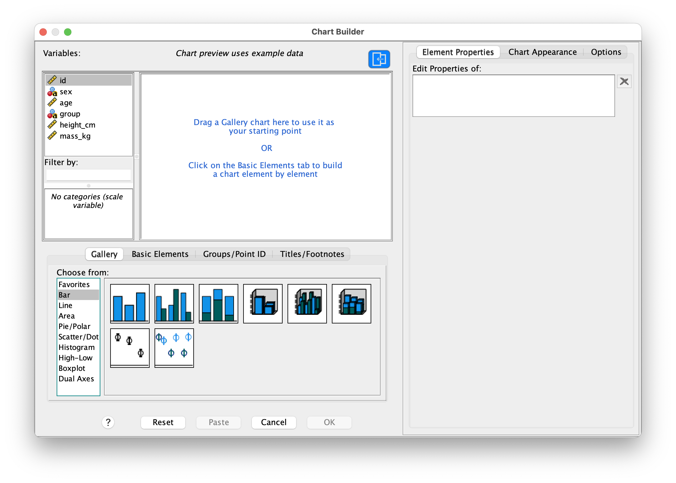
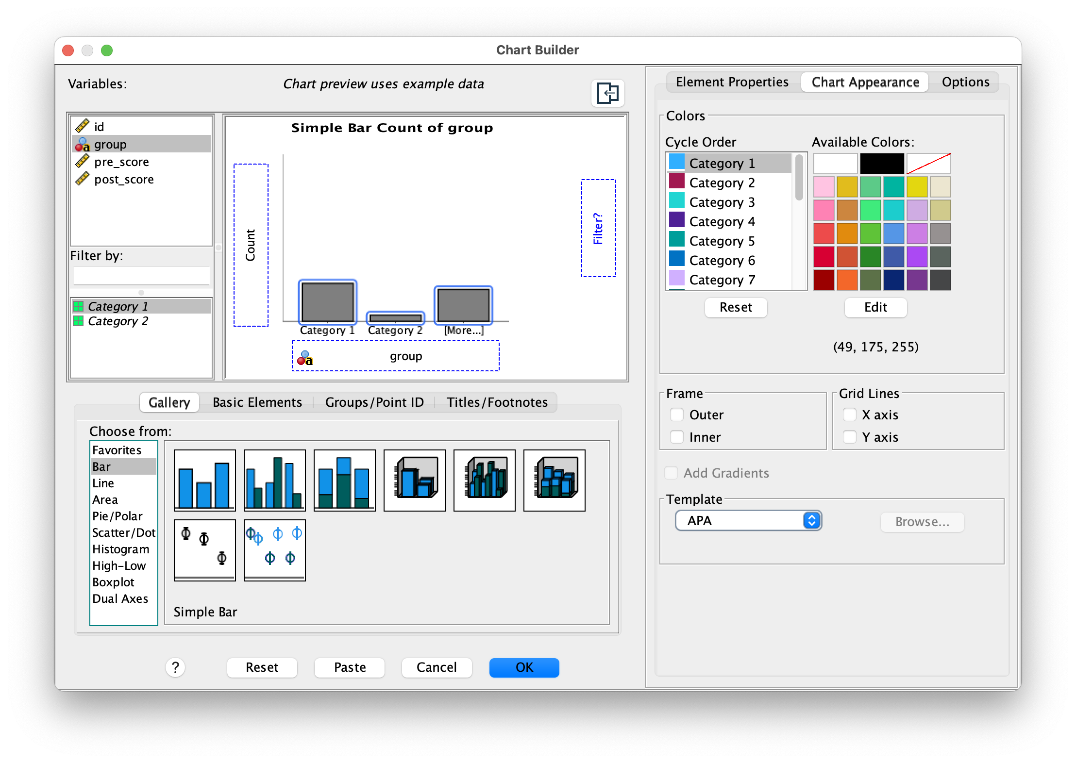
The Chart Builder uses an intuitive drag-and-drop interface that makes creating visualizations straightforward. You can preview how your chart will look and customize various elements like colors, labels, and formatting before generating the final version. While SPSS also maintains Legacy Dialogs for creating charts (found under Graphs > Legacy Dialogs), the Chart Builder offers a more visual and user-friendly approach with better preview capabilities. The legacy dialogs are still available for users who prefer the older interface or need specific chart types not yet available in Chart Builder, but for most purposes, Chart Builder provides greater flexibility and easier customization.

Figure H.5: Chart Builder Home

H.5 Datasets & File Types

SPSS works with native .sav/.zsav files and imports .csv, .xlsx, and .txt. Output is saved as .spv and can be exported to common formats like .pdf, .docx, .png, and .html.

H.6 Data Entry & Variable View

Use Variable View to define types, labels, and missing codes. Data View shows cases and variables; switch between them as you edit and review your dataset.

H.7 Opening vs. Importing Data

SPSS distinguishes between opening data files and importing data files, and understanding this difference is important for working efficiently.

H.7.1 Opening Data Files

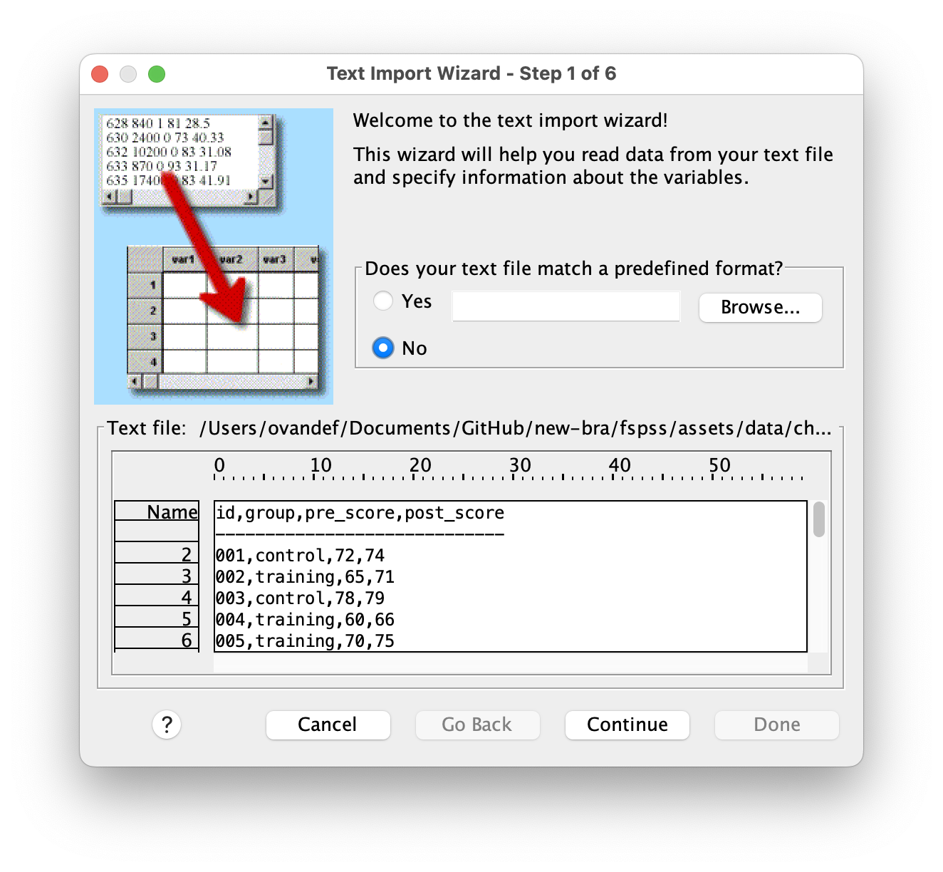
Use File > Open > Data when working with files that are already in SPSS format (.sav or .zsav) or when opening simple data files like CSV where SPSS can automatically handle the conversion. When you open a CSV file this way, SPSS recognizes the file format and launches the Text Import Wizard to help you configure how the data should be read. This is the most common approach for everyday data work.

H.7.2 Importing Data Files

Use File > Import Data when you need more control over how data from other formats (Excel, databases, text files with complex structures) are brought into SPSS. The Import Data menu provides specialized wizards for different file types:

• Excel: Handles .xlsx and .xls files with multiple worksheets
• Text Data: For delimited or fixed-width text files requiring specific configuration
• Database: Connects to external databases like SQL Server or Oracle
• Other formats: SAS, Stata, and other statistical software formats

The key distinction: Open is simpler and works for most common situations, while Import offers specialized tools for complex data sources.

H.8 Working with CSV Files

H.8.1 CSV Import Steps

To open a CSV file, go to File > Open > Data and browse to your CSV file. SPSS automatically recognizes CSV files and launches the Text Import Wizard. The wizard asks you to select the delimiter that separates values in your file—usually this is a comma, but it could be a tab, semicolon, or other character. Make sure to specify that the first row contains variable names so SPSS uses those as column headers. Take time to preview the data and confirm that SPSS has correctly identified each variable’s data type (numeric, string, etc.). Once everything looks correct, save your imported data as a .sav or .zsav file so you have a native SPSS version to work with.

Figure H.6: Import Dialog

Figure H.7: Data View After Import

H.9 Working with Excel Files

H.9.1 Excel Import

For Excel files, use File > Import Data > Excel to start the import wizard. You’ll need to select which worksheet contains your data if the Excel file has multiple sheets. The wizard allows you to specify the range of cells to import and whether the first row contains variable names. Pay special attention to columns that might contain mixed types of data (both numbers and text), as these can cause import problems if not handled correctly. Excel files with complex formatting, merged cells, or formulas may require cleanup before importing.

H.9.2 Define Variable Properties

After importing data from any source, SPSS offers a helpful tool at Data > Define Variable Properties that can save you time. This feature scans through your data values and suggests appropriate variable types, labels, and missing value codes based on what it finds. Review these suggestions carefully and apply the ones that make sense for your dataset.

H.10 Sample Datasets

You can download the practice datasets directly below:

1. athletes.csv — Instructor demonstration file

• Download: athletes.csv
• Variables: id, sex, age, group, height_cm, mass_kg, pre_score, post_score
• 20 cases; includes pre/post scores for transformation demos

2. participants.csv — Demographics and anthropometric data

• Download: participants.csv
• Variables: id, sex, age, group, height_cm, mass_kg
• 24 cases; balanced groups

3. pre_post_scores.csv — Pre/post intervention scores

• Download: pre_post_scores.csv
• Variables: id, group, pre_score, post_score
• 26 cases; includes missing values for practice

4. reaction_time_trials.csv — Repeated measures reaction times

• Download: reaction_time_trials.csv
• Variables: id, condition, rt_t1_ms, rt_t2_ms, rt_t3_ms
• 20 cases; wide format for within-subjects analysis

H.11 Saving & Exporting

H.11.1 Save Dataset

Once you’ve organized your data and performed initial transformations, it’s important to save your work in SPSS’s native format. Navigate to File > Save As and choose between .sav (standard SPSS file) and .zsav (compressed format that takes less disk space). Use descriptive filenames that include version information, such as participants_v01_cleaned.sav or study_data_20250110.sav, so you can track different iterations of your dataset as you work through analyses.

H.11.2 Export Output

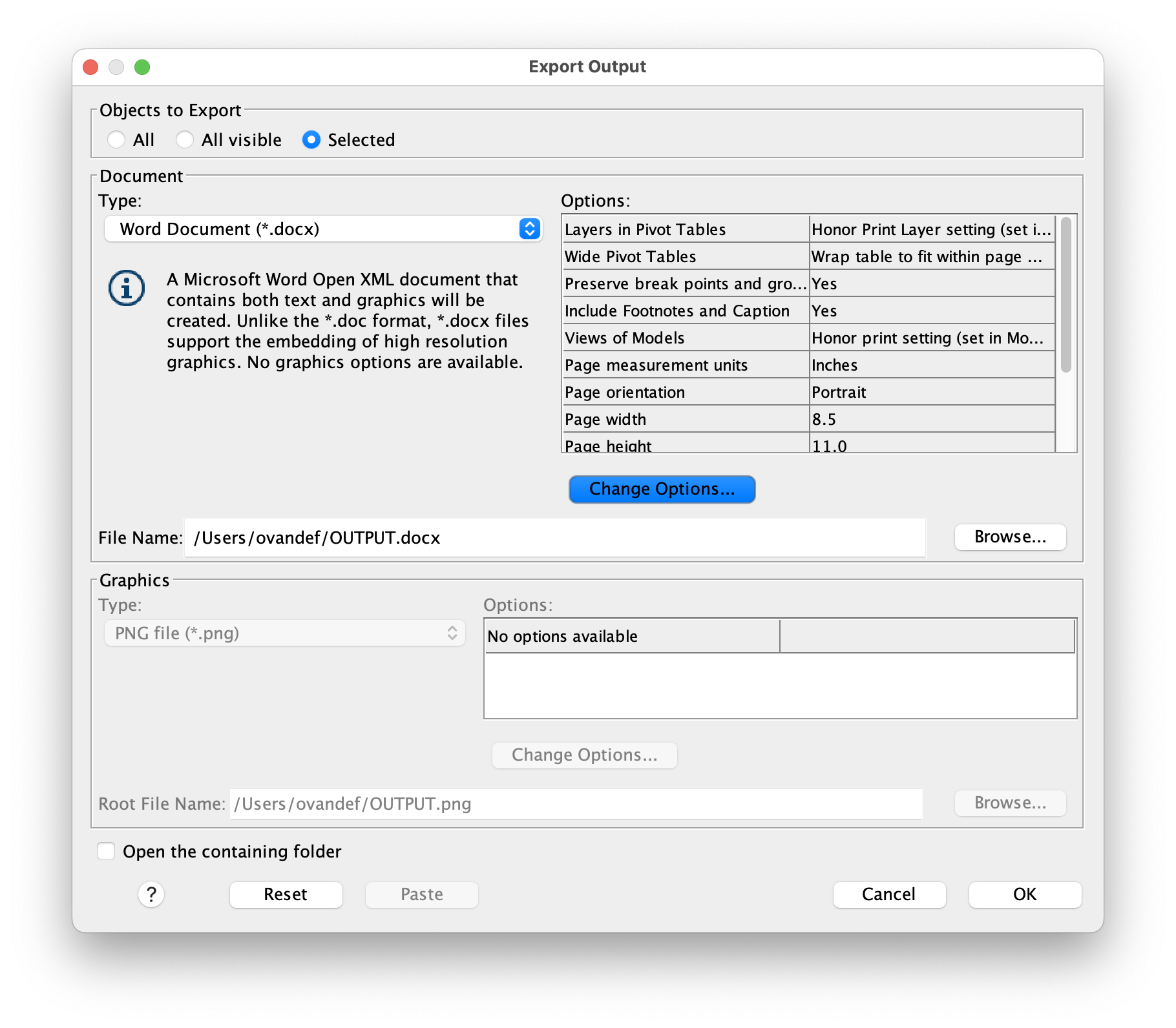
When you’re ready to share results or include them in papers and assignments, SPSS makes it easy to export your work in multiple formats. For statistical tables and summary statistics, use File > Export and select Word, PDF, or Excel format depending on your needs. For charts and figures, right-click directly on the chart in the Output Viewer and choose Export; PNG format is recommended for print publications and presentations because it maintains high quality at various sizes.

H.11.3 APA Basics

Whether you’re creating tables for a paper or assignment, follow these APA formatting conventions to ensure professional appearance. Place table titles above the table (centered and bold) and any explanatory notes below in smaller text. Keep numerical values consistent by rounding to 2 decimal places throughout your table—this creates visual consistency and makes patterns easier to spot. Use clear, descriptive variable labels rather than cryptic abbreviations, and avoid unnecessary visual elements like gridlines, excessive colors, or 3D effects that distract from the data itself.

Figure H.8: Export Dialog

H.12 Chart Builder Primer

SPSS’s Chart Builder provides an intuitive, drag-and-drop interface for creating professional visualizations. Rather than memorizing specific menu paths for each type of chart, you can experiment with different chart types and see previews in real time. This visual approach helps you choose the most appropriate visualization for your data and makes it easy to modify charts after they’re created.

H.12.1 Common Chart Types

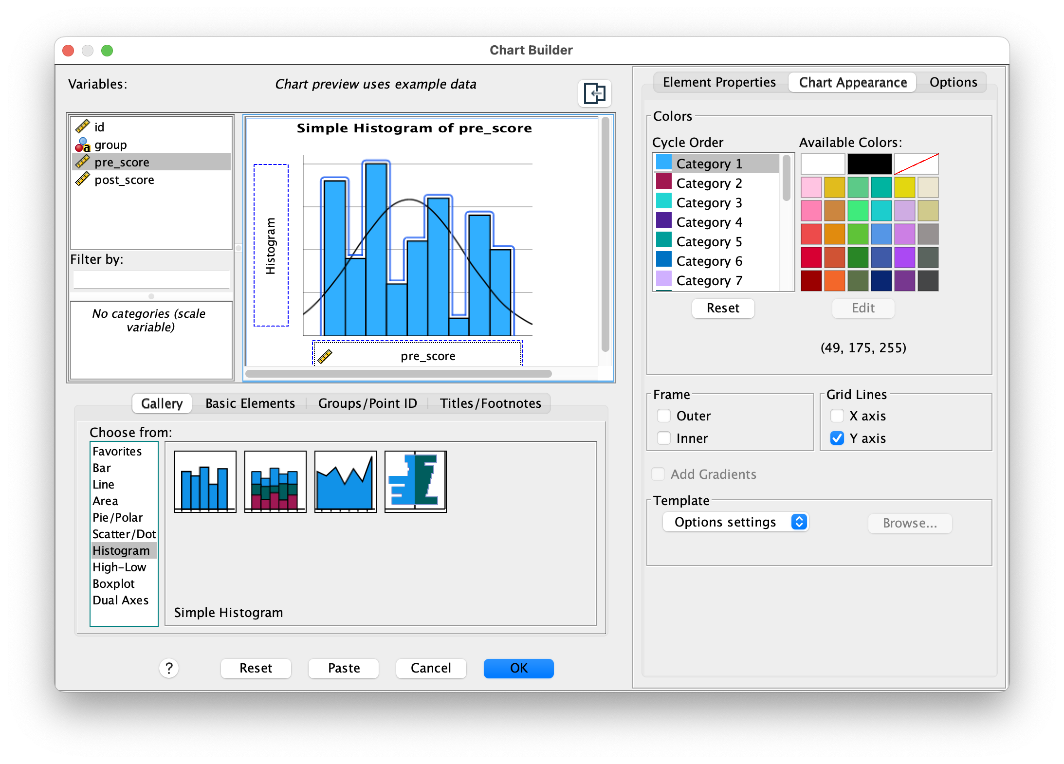
Different chart types serve different purposes depending on your data and what you want to communicate. Use a Histogram when you want to visualize the distribution of a single continuous variable—it shows you whether your data is normally distributed or skewed. A Boxplot is excellent for comparing distributions across groups; it displays the median, quartiles, and outliers all in one compact graphic. Bar Charts are useful for showing counts or mean values broken down by categories, making it easy to compare groups at a glance. A Scatterplot is the standard choice when you want to show the relationship between two continuous variables and help readers see patterns or correlations.

H.12.2 Steps

To create any chart, start by selecting Graphs > Chart Builder from the menu. You’ll see a gallery of chart types on the left; drag your chosen chart type onto the canvas in the center. Assign your variables to the appropriate axes by dragging them from the Variables list. Once the basic structure is in place, customize the appearance by adding titles, axis labels, changing colors, and adjusting fonts to match your preferences. Finally, click OK to generate the chart in the Output Viewer, where you can further refine it if needed.

Figure H.9: Chart Builder Layout

Figure H.10: Histogram Output

Figure H.11: Boxplot Output

Tip

Further reading: To learn more about effective data visualization, click here

H.13 Basic Transformations

H.13.1 Compute Variable

Often you need to create new variables based on calculations involving existing ones. SPSS’s Compute Variable feature lets you define mathematical expressions that transform your data. Access it through Transform > Compute Variable, where you can build new variables from existing ones. Common uses include creating z-scores (standardized values for comparison across variables), calculating difference or change scores (useful for pre-post designs), or summing items into composite scales. Once you define your expression, SPSS applies it to all cases in your dataset, creating a new column with the computed values.

* Compute z-score.
COMPUTE z_mass = (mass_kg - 75) / 12.
EXECUTE.

* Compute change score.
COMPUTE change = post_score - pre_score.
EXECUTE.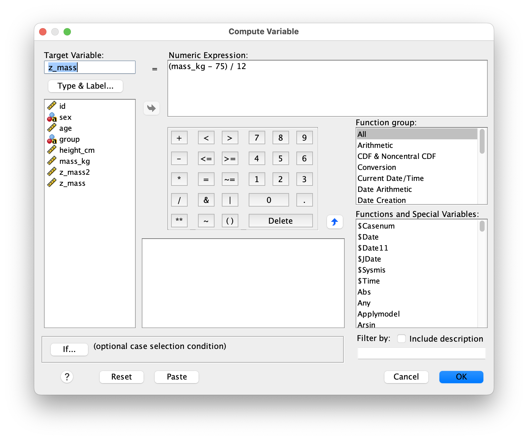

Figure H.12: Compute Dialog

H.13.2 Recode Into Different Variables

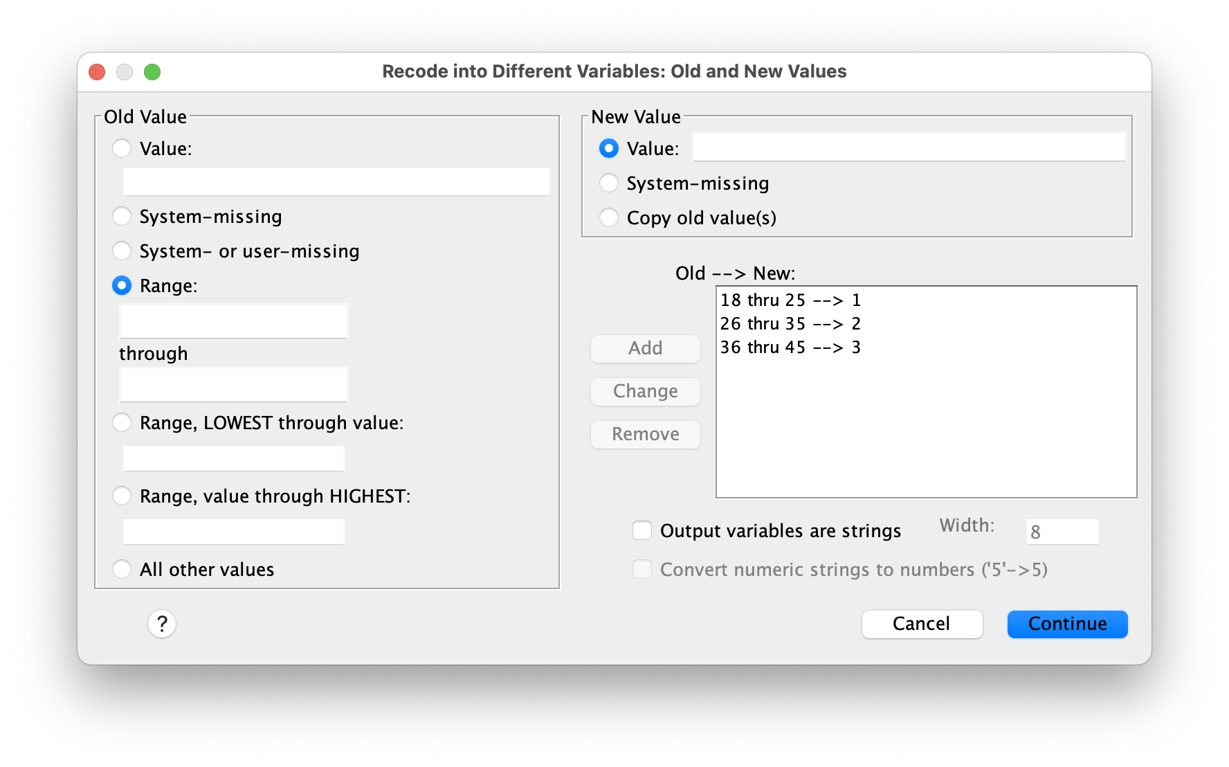
Recoding allows you to group continuous values into categories or change coding schemes while preserving your original data intact. Use Transform > Recode into Different Variables to specify how old values should map to new values. For example, you might recode age into age groups (18-25, 26-35, etc.) or recode a 5-point Likert scale into broader categories. Because you’re recoding “into different variables,” your original variable remains unchanged—SPSS creates a new variable with the recoded values, which is safer than overwriting your raw data.

* Recode age into groups.
RECODE age (18 thru 25=1) (26 thru 35=2) (36 thru 45=3) INTO age_group.
VALUE LABELS age_group 1 '18-25' 2 '26-35' 3 '36-45'.
EXECUTE.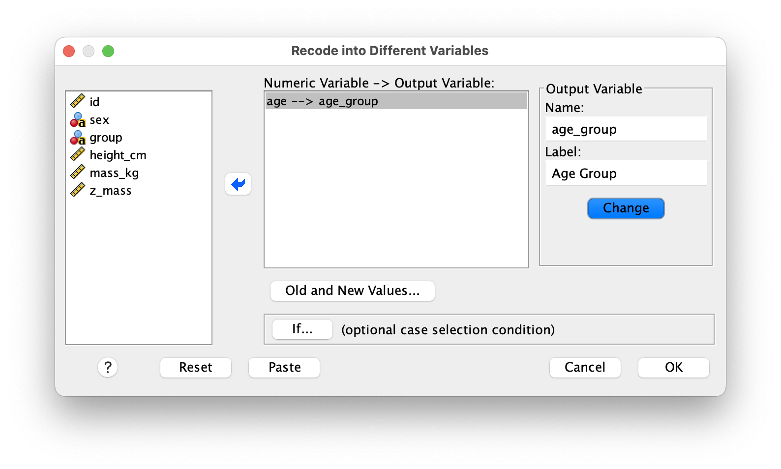

Figure H.13: Recode Dialog

Figure H.14: Recode Dialog

H.13.3 Reverse-Scoring

When creating composite scales from multiple items, you sometimes encounter items that are worded in the opposite direction—these need to be reverse-scored so that all items measure the construct in the same direction. For example, if your scale ranges from 1 to 5, reverse scoring an item means subtracting its value from 6 (one point higher than your maximum). This flips the scale so that a 1 becomes a 5 and vice versa. Always create a new variable with the reverse-scored values rather than overwriting the original item, so you maintain a record of your raw data. You can accomplish this with a simple Compute Variable expression:

* Reverse score (assuming 1-5 scale).
COMPUTE item1_rev = 6 - item1.
EXECUTE.

H.14 Syntax Basics

While SPSS’s menu-driven interface is user-friendly, syntax—the command language underlying SPSS—is essential for serious data analysis. Learning syntax might seem intimidating at first, but it offers powerful advantages that make your work more professional and reliable.

H.14.1 Why Use Syntax?

Syntax creates a permanent record of every step you took, allowing you to reproduce your exact analyses weeks or months later—critical when you need to verify results or make small adjustments to your work. You can also document your thinking by adding comments throughout your syntax file, explaining why you chose specific approaches or noting data issues you discovered. Beyond reproducibility, syntax lets you batch process multiple operations at once, saving time when you have repetitive tasks or need to apply the same transformations to multiple variables.

H.14.2 Creating Syntax

There are several ways to build a syntax file. The easiest approach for beginners is to use the menu system as you normally would, but instead of clicking OK to execute the command, click Paste. This copies the equivalent syntax command to a syntax editor window, where you can review, modify, and save it. As you become more comfortable with syntax, you can also type commands directly into the Syntax Editor, and many experienced users find this faster than navigating menus. Always save your syntax files with a .sps extension so they’re easy to identify and can be opened reliably on any system.

H.14.3 Running Syntax

To run your syntax commands, highlight the lines you want to execute (or leave everything highlighted to run the entire file), then click the Run button (green arrow) in the toolbar or use the keyboard shortcut Cmd+R on Mac or Ctrl+R on Windows. SPSS will process your commands in order and generate output in the Output Viewer. An important note: after any commands that modify your data (like Compute, Recode, or Select If), include the EXECUTE. statement to tell SPSS to finalize the changes before moving to the next step. Some users add EXECUTE. at the end of every section for extra clarity.

* Load dataset.
GET FILE='assets/data/ch01/participants.sav'.
DATASET NAME participants.

* Descriptive statistics.
DESCRIPTIVES VARIABLES=height_cm mass_kg
  /STATISTICS=MEAN STDDEV MIN MAX.

EXECUTE.

H.14.4 Annotation

Good comments are invaluable when you return to your syntax weeks later or when a colleague needs to understand your work. Use a single asterisk * at the beginning of a line for single-line comments (SPSS will ignore everything from the asterisk to the period). For longer explanations that span multiple lines, use /* */ to wrap your comment. At the very top of your syntax file, always include a header documenting the purpose of the analysis, the date it was created or last modified, and who wrote it. These simple practices make your work look professional and help prevent confusion or mistakes when revisiting old analyses.

H.15 Data Integrity Checks

Before you begin any analysis, it’s essential to verify that your data has been entered and imported correctly. Data integrity checks help you catch errors early—before they compromise your results. These checks typically look for out-of-range values, suspicious patterns, and missing data issues.

H.15.1 Check Ranges

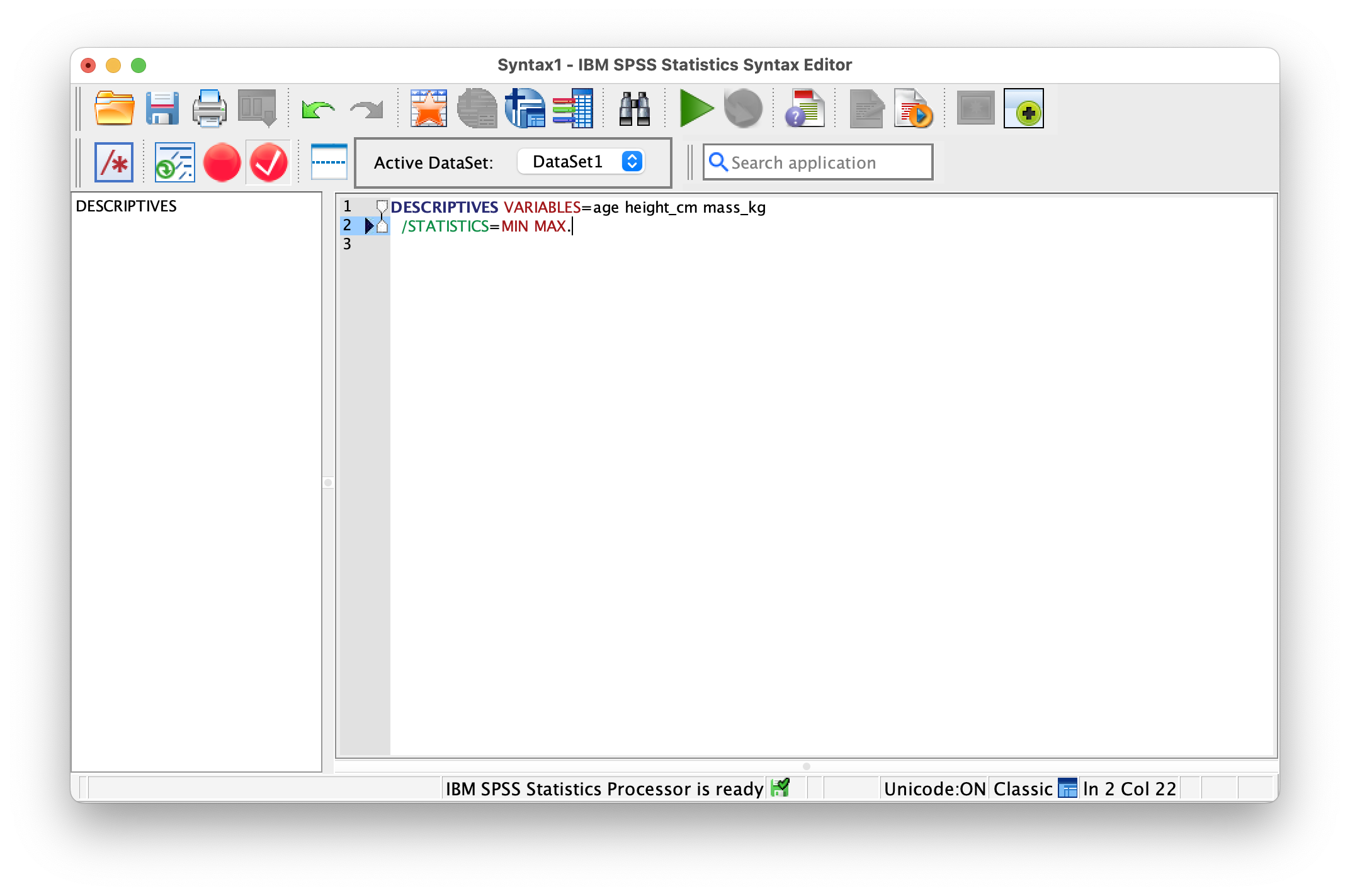
Run a simple Descriptive Statistics command to see the minimum and maximum values for your numeric variables. This is your first line of defense against data entry errors. Look carefully at these values—if someone entered a height of 999 cm or an age of -5, these errors will be obvious:

DESCRIPTIVES VARIABLES=age height_cm mass_kg
  /STATISTICS=MIN MAX.

Any impossible values should be investigated. They might be legitimate outliers, data entry errors, or missing value codes that weren’t properly configured.

H.15.2 Missing Data Patterns

Understanding patterns of missing data is crucial because they can affect your analyses in subtle ways. Use the Frequencies command to examine which cases have missing values and whether the missingness follows any pattern:

FREQUENCIES VARIABLES=pre_score post_score
  /FORMAT=NOTABLE
  /STATISTICS=MISSING.

For example, if all missing values in a post_score variable come from one group, that suggests a systematic problem rather than random missing data. This information will help you decide whether to use listwise deletion, imputation, or other strategies for handling missing values.

H.15.3 Identify Duplicates

Occasionally you may have duplicate rows in your dataset—cases that were entered twice by mistake. SPSS provides a tool at Data > Identify Duplicate Cases that scans your data and highlights potential duplicates. Specify your ID variable so SPSS knows how to match cases, and it will flag duplicates for your review. You then decide whether to keep the first occurrence, the last occurrence, or review each duplicate manually to determine which version is correct. This step is particularly important if you’ve merged multiple data sources.

H.15.4 Sort and Select Cases

As you work with your data, you may want to organize it by certain variables or focus on a subset of cases. Use the Sort Cases command to arrange your data in a specific order, which is helpful for spotting patterns or preparing data for specific analyses. When you only want to analyze a portion of your data (for example, just the training group), use Select If to temporarily filter the dataset:

* Sort by ID.
SORT CASES BY id.

* Select cases for analysis.
SELECT IF (group = 'training').
EXECUTE.

Note that Select If doesn’t delete cases—it just marks them as excluded from analyses. You can always clear the selection later to work with the full dataset again.

H.16 Preferences & Defaults

SPSS offers extensive customization options to tailor the interface and output to your preferences and workflow. Taking time to configure these settings will save you effort throughout the course.

H.16.1 Display Options

Navigate to Edit > Options > Output to control how SPSS displays your results. You can choose whether tables show variable names (compact but cryptic) or variable labels (more readable if you’ve entered descriptive labels). Set your default number of decimal places displayed—this affects readability and follows conventions (typically 2 decimals for most statistical output). You can also adjust the scientific notation threshold, which determines when SPSS switches to exponential notation for very large or very small numbers.

H.16.2 File Paths

Use Edit > Options to set your default locations for opening and saving files. This saves you from repeatedly navigating to the same folder. In your syntax files, use relative paths (like assets/data/ch01/participants.sav) rather than absolute paths (like /Users/yourname/Documents/...). Relative paths are portable—if you move your project folder to a different location or share it with someone else, the syntax will still work.

H.16.3 Output Style

Edit > Options > Pivot Tables lets you customize how tables appear in your output. SPSS includes an APA style option that automatically formats tables according to American Psychological Association standards—this is ideal for coursework and research papers. You can also adjust fonts and cell formatting to suit your preferences or match a specific publication style.

H.17 Quick Practice Tasks

These hands-on exercises will help you apply the concepts covered in this chapter. Work through each task systematically, documenting your steps as you go. These tasks build on each other, so complete them in order.

1. Project Setup with Google Drive: Create a well-organized folder structure in your Google Drive to maintain all course materials in one centralized, accessible location. In your Google Drive, create a main folder called SPSS_Course (or similar). Inside this main folder, create four subfolders: data (for raw and processed data files), syntax (for your .sps script files), output (for saved SPSS output files), and figures (for exported charts and graphs).

TipOptional: Install Google Drive for Desktop (Recommended)

Install Google Drive for Desktop on your computer so these folders sync automatically and appear as a regular folder on your Mac/PC. Once synced, you can access these folders through Finder (Mac) or File Explorer (Windows) just like any other local folder. In SPSS, this synced folder by going to File > Change Working Directory, thenset your working directory to point to this synced folder by going to File > Change Working Directory and navigating to the Google Drive folder on your computer. This setup ensures your work is automatically backed up to the cloud and accessible from any device.

2. Data Import and Initial Inspection: Download the athletes.csv file provided above and save it to your data subfolder within your Google Drive SPSS_Course folder. Open SPSS and import this file using File > Open > Data, selecting the CSV format. After importing, examine the Data View to ensure all variables loaded correctly. Check that numeric variables appear as numbers (not text) and that there are no obvious formatting issues. Save the file as athletes.sav in your data folder.

3. Configure Metadata: Switch to Variable View and systematically define metadata for all variables. Add meaningful variable labels that describe what each variable measures (e.g., “Athlete height in centimeters” for height_cm, “Pre-test score” for pre_score, “Post-test score” for post_score). For categorical variables like sex and group, define value labels (M = ‘Male’, F = ‘Female’ for sex; control = ‘Control’, training = ‘Training’ for group). Set the appropriate measurement level for each variable: Scale for continuous variables, Ordinal for ordered categories, and Nominal for unordered categories.

4. Data Transformation: Create two new computed variables. First, create bmi from height and mass using the formula: BMI = mass_kg / (height_cm/100)². Second, create a change_score variable by subtracting pre_score from post_score to see training improvements. Use Transform > Compute Variable for both. Then, use Transform > Recode into Different Variables to create age groups from the continuous age variable. Create categories: 18-25, 26-35, 36-45, 46+. Remember to add value labels to your new age_group variable.

5. Visual Data Exploration: Open the Chart Builder (Graphs > Chart Builder) and create two visualizations. First, create a histogram of the mass_kg variable to examine its distribution—look for whether it appears normally distributed or skewed. Second, create a boxplot comparing mass_kg across the group variable to see if there are differences between control and training groups. Export both charts as image files to your figures folder using File > Export after right-clicking each chart.

6. Syntax Documentation: This is crucial for reproducibility. Open a new Syntax Editor (File > New > Syntax). Go back through each of the steps above (import, compute, recode, chart) and use the Paste button instead of OK to capture the syntax for each operation. Organize your syntax file with clear comments explaining each section. Add EXECUTE. commands after data transformations. Save this file as chapter01_practice.sps in your syntax folder. Close your dataset without saving, then run your entire syntax file from start to finish to verify it reproduces all your work.

7. Data Quality Control: Run comprehensive data integrity checks. Use Descriptive Statistics to examine the minimum and maximum values for age, height_cm, and mass_kg—verify that all values fall within plausible ranges (e.g., height between 140-210 cm). Use Frequencies to check for missing data patterns. Finally, use Data > Identify Duplicate Cases with the id variable to ensure no participants were entered twice. Document any issues you find and how you resolved them.

Practice Solutions

Task 1: Project Setup with Google Drive

1. Open your web browser and go to drive.google.com
2. Sign in with your Google account (or create one if needed)
3. Click the + New button on the left side
4. Select New folder
5. Name it SPSS_Course and click Create
6. Click into the newly created SPSS_Course folder
7. Create four subfolders by repeating the New folder process:
   • data
   • syntax
   • output
   • figures

TipOptional: Install Google Drive for Desktop (Recommended)

Installing Google Drive for Desktop allows you to access your Google Drive files directly through Finder (Mac) or File Explorer (Windows), making it much easier to work with SPSS. Files sync automatically between your computer and the cloud.

1. Visit google.com/drive/download
2. Download the appropriate version for your operating system
3. Run the installer and follow the on-screen instructions
4. Sign in with the same Google account you used to create the folders
5. In the settings, ensure “Stream files” or “Mirror files” is enabled (Mirror is recommended for SPSS work)
6. Once installed, Google Drive will appear in your Finder (Mac) or File Explorer (Windows) sidebar
7. Navigate to Google Drive > SPSS_Course to see your synced folders

Benefits: Any files you save to the SPSS_Course folder will automatically sync to the cloud. You can access these files from any computer or through the Google Drive website. If you work on a different computer, just install Google Drive for Desktop there and sign in with the same account—all your files will be available.

8. Open SPSS
9. Go to File > Change Working Directory
10. Navigate to your Google Drive folder:
    • If you installed Google Drive for Desktop: /Users/[YourName]/Google Drive/SPSS_Course on Mac or G:\My Drive\SPSS_Course on Windows
    • If using browser-only: Download files from Google Drive to a local folder and navigate to that folder
11. Click OK to set this as your working directory
12. To verify, check that the SPSS title bar or status shows your chosen path

NoteOptional: Syntax Version

* No syntax needed - this is folder and system setup
* Working directory can be set via File > Change Working Directory
* Or you can use CD command:
CD '/Users/[YourName]/Google Drive/SPSS_Course'.

Task 2: Data Import

1. Open SPSS and go to File > Open > Data
2. Navigate to your data subfolder and select athletes.csv
3. The Text Import Wizard will open automatically
4. In Step 1, verify that “Delimited” is selected and click Next
5. In Step 2, check “Comma” as the delimiter and ensure “First case of data starts on line” is set to 2 (since row 1 contains variable names)
6. In Step 3, verify the variable names are correct (id, sex, age, group, height_cm, mass_kg, pre_score, post_score)
7. In Step 4, review the data preview to ensure all columns look correct
8. Click Finish to import the data
9. Immediately go to File > Save As, choose “SPSS Statistics (*.sav)” as the file type, name it athletes.sav, and save it in your data folder

NoteOptional: Syntax Version

GET DATA
  /TYPE=TXT
  /FILE='data/athletes.csv'
  /DELIMITERS="," 
  /QUALIFIER='"'
  /ARRANGEMENT=DELIMITED
  /FIRSTCASE=2
  /VARIABLES=
  id F3.0
  sex A1
  age F2.0
  group A8
  height_cm F5.0
  mass_kg F5.0
  pre_score F4.1
  post_score F4.1.
CACHE.
EXECUTE.

SAVE OUTFILE='data/athletes.sav'
  /COMPRESSED.

Task 3: Configure Metadata

1. Click the Variable View tab at the bottom of the Data Editor window
2. For each variable, click in the Label column and add descriptive labels:
   • id: “Athlete identification number”
   • sex: “Biological sex”
   • age: “Age in years”
   • group: “Experimental group assignment”
   • height_cm: “Height in centimeters”
   • mass_kg: “Body mass in kilograms”
   • pre_score: “Pre-test performance score”
   • post_score: “Post-test performance score”
3. For the sex variable, click in the Values column, then click the small button that appears
4. In the Value Labels dialog, add: Value = M, Label = “Male”, click Add; then Value = F, Label = “Female”, click Add, then OK
5. For the group variable, repeat: Value = control, Label = “Control”, click Add; Value = training, Label = “Training”, click Add, then OK
6. For the Measure column, set:
   • id, age, height_cm, mass_kg, pre_score, post_score: Scale
   • sex, group: Nominal
7. Save your file (Ctrl+S or Cmd+S)

NoteOptional: Syntax Version

VARIABLE LABELS
  id 'Athlete identification number'
  sex 'Biological sex'
  age 'Age in years'
  group 'Experimental group assignment'
  height_cm 'Height in centimeters'
  mass_kg 'Body mass in kilograms'
  pre_score 'Pre-test performance score'
  post_score 'Post-test performance score'.

VALUE LABELS
  sex 'M' 'Male' 'F' 'Female'
  /group 'control' 'Control' 'training' 'Training'.

VARIABLE LEVEL
  id age height_cm mass_kg pre_score post_score (SCALE)
  /sex group (NOMINAL).
EXECUTE.

Task 4: Data Transformation

Creating the BMI variable: 1. Go to Transform > Compute Variable 2. In the Target Variable box, type: bmi 3. In the Numeric Expression box, type: mass_kg / ((height_cm/100) ** 2) 4. Click OK 5. Switch to Variable View, find the new bmi variable, and add the label “Body Mass Index” in the Label column

Creating the change score variable: 1. Go to Transform > Compute Variable again 2. In the Target Variable box, type: change_score 3. In the Numeric Expression box, type: post_score - pre_score 4. Click OK 5. Switch to Variable View, find the new change_score variable, and add the label “Change in performance score” in the Label column

Creating age groups: 1. Go to Transform > Recode into Different Variables 2. Select age from the left list and move it to the Input Variable -> Output Variable box 3. In the Output Variable section, type age_group as the Name 4. Click Change to confirm the new variable name 5. Click Old and New Values 6. In the Old Value section, select “Range” and enter 18 through 25, then in New Value enter 1, click Add 7. Repeat for: 26 through 35 = 2, 36 through 45 = 3, 46 through Highest = 4 8. Click Continue, then OK 9. Switch to Variable View, find age_group, and add the label “Age group category” 10. In the Values column for age_group, add: 1=‘18-25’, 2=‘26-35’, 3=‘36-45’, 4=‘46+’ 11. Set Measure to Ordinal

NoteOptional: Syntax Version

COMPUTE bmi = mass_kg / ((height_cm/100) ** 2).
VARIABLE LABELS bmi 'Body Mass Index'.
EXECUTE.

COMPUTE change_score = post_score - pre_score.
VARIABLE LABELS change_score 'Change in performance score'.
EXECUTE.

RECODE age (18 thru 25=1) (26 thru 35=2) (36 thru 45=3) (46 thru HIGHEST=4)
  INTO age_group.
VARIABLE LABELS age_group 'Age group category'.
VALUE LABELS age_group
  1 '18-25'
  2 '26-35'
  3 '36-45'
  4 '46+'.
VARIABLE LEVEL age_group (ORDINAL).
EXECUTE.

Task 5: Visual Data Exploration

Creating a histogram: 1. Go to Graphs > Chart Builder 2. If prompted, click OK on the variable properties dialog 3. In the Gallery tab on the left, select Histogram 4. Drag the simple histogram icon to the canvas area 5. From the Variables list, drag mass_kg to the X-Axis drop zone 6. Click OK to generate the chart 7. In the Output Viewer, right-click the histogram and select Export 8. Choose PNG format, navigate to your figures folder, name it histogram_mass.png, and click Save

Creating a boxplot: 1. Go to Graphs > Chart Builder 2. In the Gallery, select Boxplot 3. Drag the simple boxplot icon to the canvas 4. Drag mass_kg to the Y-Axis drop zone 5. Drag group to the X-Axis drop zone 6. Click OK to generate the chart 7. Right-click the boxplot in the Output Viewer, select Export 8. Save as PNG in your figures folder with the name boxplot_mass_by_group.png

NoteOptional: Syntax Version

GRAPH
  /HISTOGRAM=mass_kg
  /TITLE='Distribution of Body Mass'.

GRAPH
  /BOXPLOT=mass_kg BY group
  /TITLE='Body Mass by Group'.

Task 6: Syntax Documentation

1. Go to File > New > Syntax

2. In the empty syntax editor, create a header with comments:

   * ============================================
   * Chapter 1 Practice Exercises
   * Author: [Your Name]
   * Date: [Today's Date]
   * Purpose: Complete workflow from import to QC
   * ============================================

3. Now, repeat each of the previous tasks (import, compute, recode, charts) but instead of clicking OK in each dialog, click Paste

4. The syntax will be copied to your syntax editor window

5. Add comments using * before each section to explain what you’re doing

6. Add EXECUTE. after any data transformation commands

7. Save the syntax file as chapter01_practice.sps in your syntax folder (File > Save As)

8. To test it: Close your data file without saving changes (if asked)

9. Highlight all the syntax (Ctrl+A or Cmd+A) and click the green Run arrow (or press Ctrl+R / Cmd+R)

10. Verify that all output appears correctly in the Output Viewer

Task 7: Data Quality Control

Checking ranges: 1. Go to Analyze > Descriptive Statistics > Descriptives 2. Move age, height_cm, and mass_kg to the Variable(s) box 3. Click Options and ensure “Mean”, “Std. deviation”, “Minimum”, and “Maximum” are checked 4. Click Continue, then OK 5. Review the output table—check that minimum and maximum values are within plausible ranges (e.g., age 18-60, height 140-210 cm, mass 45-120 kg)

Checking missing data patterns: 1. Go to Analyze > Descriptive Statistics > Frequencies 2. Move all variables to the Variable(s) box 3. Click Statistics and check “Missing” 4. Uncheck any default statistics you don’t need 5. Click Continue 6. Click Format, select “Suppress tables with more than N categories” and set to 0 (this hides the frequency tables) 7. Click Continue, then OK 8. Review the output to see how many missing values exist for each variable

Identifying duplicates: 1. Go to Data > Identify Duplicate Cases 2. Move id to the Define matching cases by box 3. Select “First case in each group” under Cases to exclude 4. Click OK 5. SPSS will create a new variable showing whether each case is a duplicate (PrimaryLast) 6. Review the output—if no duplicates exist, all cases should be marked as “Primary” 7. You can delete the PrimaryLast variable after confirming no duplicates exist

NoteOptional: Syntax Version

* Check ranges
DESCRIPTIVES VARIABLES=age height_cm mass_kg
  /STATISTICS=MIN MAX MEAN STDDEV.

* Check for missing data
FREQUENCIES VARIABLES=ALL
  /FORMAT=NOTABLE
  /STATISTICS=MISSING.

* Identify duplicate IDs
SORT CASES BY id.
AGGREGATE
  /OUTFILE=* MODE=ADDVARIABLES
  /BREAK=id
  /id_count=N.
FREQUENCIES VARIABLES=id_count.
SELECT IF (id_count = 1).
EXECUTE.

H.18 Common Pitfalls

• Type Mismatches: Numbers imported as strings → failed analyses
• Missing Handling: Treating user-missing as valid; unintended listwise deletion
• Value Labels: Misaligned codes and labels; inconsistent order
• Paths: Hard-coded absolute paths break when project moves
• Overwriting: Recode into same variable without backup
• Manual Edits: Changing output tables without updating dataset or syntax

H.19 Readiness Checklist

• SPSS 31 installed and licensed
• Project folders organized (data, syntax, output, figures)
• Sample datasets imported and saved as .sav
• Variable types, labels, and missing values defined
• At least one Compute and one Recode completed
• Histogram and boxplot created and exported
• Master .sps script runs end-to-end without errors
• Range and missing checks performed; no duplicates or invalid values

H.20 Using SPSS 31 in Apporto

H.20.1 What is Apporto?

Apporto is a cloud-based virtual desktop platform that provides access to software applications through your web browser. For this course, you’ll use Apporto to run SPSS 31 without needing to install it on your personal computer. This ensures everyone has access to the same version of SPSS regardless of their device (Windows, Mac, Chromebook, etc.).

H.20.2 Accessing Apporto

1. Open your web browser and navigate to the Apporto login page link provided in Canvas
2. Log in using your institutional credentials
3. Once logged in, you’ll see a virtual desktop environment

H.20.3 Launching SPSS 31

1. On the Apporto desktop, look for the SPSS icon (it may be in a folder labeled “Statistics” or “Software”)
2. Double-click the SPSS 31 icon to launch the application
3. SPSS may take a moment to load - be patient during the initial startup

H.20.4 Working with Files

• Opening Files: Use File → Open → Data to load SPSS data files (.sav)
• Importing Data: Use File → Import Data for Excel, CSV, or other formats
• Creating New Files: Start with a blank dataset using File → New → Data

H.20.5 Saving Your Work

Important

Always save your work regularly! Apporto sessions may timeout, and unsaved work will be lost.

1. Use File → Save As to save your SPSS data file (.sav)
2. Save output files (.spv) separately using File → Export in the Output Viewer
3. Files are typically saved to your personal network drive or OneDrive within Apporto

H.20.6 Downloading and Uploading Files

H.20.6.1 Uploading Files to Apporto

To transfer files from your local computer to Apporto:

1. In the Apporto interface, the file manager opens to your Desktop by default
2. Click the Upload button on the main top toolbar (it looks like an upward arrow)
3. In the file picker dialog that opens, select the file(s) from your local computer
4. Wait for the upload to complete - you’ll see a progress indicator
5. Once uploaded, you can open the file in SPSS using File → Open → Data

H.20.6.2 Downloading Files from Apporto

To transfer files from Apporto to your local computer:

1. In the Apporto interface, the file manager opens to your Desktop by default (where your files are typically saved)
2. Select the SPSS data file (.sav) or output file (.spv) you want to download
3. Click the Download button on the main top toolbar (it looks like a downward arrow)
4. The file will be saved to your local computer’s Downloads folder
5. You can then move the file to your preferred location on your computer

Tip

Keep your files organized by creating assignment-specific folders in Apporto. This makes it easier to find and manage your work.

H.20.7 Best Practices

• Browser Compatibility: Use Chrome, Firefox, or Edge for best performance
• Internet Connection: A stable internet connection is essential
• Session Timeouts: Apporto sessions may disconnect after periods of inactivity
• File Organization: Create folders for each assignment to keep your work organized

H.20.8 Troubleshooting

• SPSS Won’t Launch: Try refreshing your browser or restarting your Apporto session
• Slow Performance: Close unnecessary applications in Apporto
• File Access Issues: Ensure you’re saving to the correct location (usually your network drive)
• Connection Problems: Check your internet connection and try reconnecting to Apporto

If you encounter persistent issues, contact your instructor or IT support for assistance.

H.20.9 Additional Resources

• Apporto User Guide (available through your institution)
• SPSS Help: Press F1 within SPSS for context-sensitive help
• Course materials and video tutorials on SPSS usage