18  Quantifying Reliability in Movement Science

Measurement precision, ICC, SEM, MDC, and the Bland-Altman method

Tip💻 Analytical Software & SPSS Tutorials

A Note on By-Hand Calculations: The purpose of this book is not to teach tedious by-hand statistical calculations. Modern researchers run these analyses using major software packages. While we provide the underlying equations for conceptual understanding, we strongly recommend relying on software for computation to avoid errors and save time.

Please direct your attention to the SPSS Tutorial: Reliability Analysis in the appendix for step-by-step instructions on computing ICC, SEM, MDC, and Bland-Altman limits of agreement using SPSS output!

18.1 Chapter roadmap

Every statistical procedure in this textbook — from the independent t-test to ANCOVA — rests on a silent assumption that has never been stated explicitly: that the measurements entering the analysis actually measure what they are supposed to measure, and that they do so consistently. A dynamometer reading of 80 kg means nothing if the same athlete tested five minutes later would register 74 kg. A sprint time of 3.82 seconds is uninterpretable if the measurement protocol is so variable that two consecutive trials on the same day routinely differ by half a second. Before researchers can make meaningful inferences about group differences, treatment effects, or individual change, they must establish that their instruments and protocols produce consistent, reproducible results — that is, that their measurements are reliable.

Reliability is the degree to which a measurement produces the same result when applied repeatedly to the same entity under the same conditions^[1,2]. It is not a fixed property of a measuring instrument in isolation but of an instrument applied through a particular protocol to a particular population. A maximal isometric dynamometer test may be highly reliable when administered by a trained assessor following a standardized warm-up, and poorly reliable when administered ad hoc in a busy clinical setting. Reliability is always estimated from data, never assumed — and it must be reported alongside every set of measurements that will be used for inference.

This chapter introduces the four core tools for quantifying reliability in movement science: the Intraclass Correlation Coefficient (ICC), the Standard Error of Measurement (SEM), the Minimal Detectable Change (MDC), and the Bland-Altman method of limits of agreement. Each tool answers a different question, and together they provide a complete picture of measurement precision. The examples draw on the core_session.csv dataset, using the control group’s pre-test and mid-test assessments as a test-retest dataset — a design in which participants complete the same assessment twice under equivalent conditions with no intervening intervention.

18.2 Learning objectives

By the end of this chapter, you will be able to:

• Distinguish between reliability and validity, and explain why both are necessary for valid inference.
• Identify and describe the major sources of measurement error in movement science.
• Select and interpret the appropriate ICC model (ICC(1,1), ICC(2,1), ICC(3,1)) for a given reliability study design.
• Apply the Koo and Li (2016) benchmarks to classify ICC values as poor, moderate, good, or excellent.
• Compute and interpret the SEM and explain what it represents in the original measurement units.
• Calculate and apply the MDC₉₅ to determine whether an observed change in an individual exceeds measurement noise.
• Construct and interpret a Bland-Altman plot, including the bias and limits of agreement.
• Explain how poor reliability attenuates statistical effects and reduces the power of group comparisons.
• Report reliability analyses in APA style.

18.3 Workflow for a reliability study

Use this sequence when quantifying the reliability of a measurement instrument or protocol:

1. Design the study — same participants, same protocol, same assessor (or multiple assessors if inter-rater reliability is the focus), two or more occasions with no intervening intervention.
2. Restructure data to wide format (one column per test occasion).
3. Select the appropriate ICC model based on whether raters are random or fixed, and whether absolute agreement or consistency is the target.
4. Run the ICC in SPSS (Analyze → Scale → Reliability Analysis) and record the ICC value and 95% CI.
5. Compute SEM from the ICC and pooled SD (available from the Statistical Calculators appendix or SPSS 31+).
6. Compute MDC₉₅ from the SEM.
7. Construct a Bland-Altman plot to inspect for systematic bias and heteroscedasticity.
8. Report ICC with 95% CI, SEM, MDC₉₅, and Bland-Altman bias and limits of agreement.

18.4 Reliability versus validity

Reliability and validity are related but distinct properties of a measurement. Reliability refers to consistency — does the measurement produce the same result when repeated? Validity refers to accuracy — does the measurement actually capture the construct it is intended to measure? A body composition scale that consistently reads 5 kg above a person’s true mass on every weighing is highly reliable (consistent) but not valid (inaccurate). A sport psychologist’s subjective rating of athlete anxiety may have modest reliability (two raters might disagree) but reasonably good construct validity if the ratings correlate strongly with established anxiety questionnaires.

Reliability is a necessary but not sufficient condition for validity. A measurement that is not reliable cannot be valid — if it gives different results every time, it cannot consistently reflect the true underlying construct. But a reliable measurement can still be invalid if it consistently measures the wrong thing. In movement science, both properties must be evaluated: reliability through test-retest designs or inter-rater agreement studies, and validity through comparisons against gold-standard criteria, construct validation, or logical argument^[1,2].

NoteReal example: Reliable but invalid?

Resting heart rate measured by palpation (manually counting beats at the wrist) might be highly reliable between two experienced clinicians — both consistently count 68 bpm in the same patient. But if a concurrent Holter monitor recording shows 74 bpm, the palpation method is reliable but systematically biased toward underestimation. Movement science researchers must report both reliability and criterion validity when introducing a new measurement protocol, especially for field assessments that substitute for laboratory gold standards.

18.5 Sources of measurement error

Every measurement contains some degree of error — the difference between the observed score and the participant’s true underlying value. Measurement error can be broadly classified into two types. Systematic error (or bias) shifts all measurements in the same direction by a roughly constant amount: a miscalibrated force plate that reads 5 N higher than true across all trials, or a learning effect that makes performance slightly better on the second test occasion than the first regardless of any intervention. Systematic error affects validity more than reliability — it inflates or deflates scores consistently. Random error is unpredictable fluctuation around the true score: biological variability in muscle activation, day-to-day fluctuations in motivation and fatigue, minor changes in equipment positioning, or inconsistencies in the assessor’s technique. Random error directly inflates the error term in statistical analyses and is the primary target of reliability quantification^[1,3].

In a pretest–posttest design, poor reliability is particularly damaging. If a strength test has an SEM of 5 kg, then a participant whose true strength improved by 3 kg might appear to have gained anywhere from −7 to +13 kg on measurement alone. This noise not only obscures individual change but inflates the within-group variance used as the error term in ANOVA and ANCOVA, reducing statistical power for every group comparison. The connection is direct and quantitative: as reliability decreases, the correlation between true and observed scores decreases, effect sizes are attenuated toward zero, and sample size requirements increase^[2,4].

18.6 Intraclass Correlation Coefficient

18.6.1 What ICC measures

The ICC is the primary reliability statistic in movement science. Conceptually, it is the proportion of total observed variance that is attributable to true between-person differences, rather than to measurement error:

\[\text{ICC} = \frac{\sigma^2_{\text{participants}}}{\sigma^2_{\text{participants}} + \sigma^2_{\text{error}}}\]

When all participants score identically across test occasions (no error), ICC = 1.00. When the variance across occasions is as large as the variance among participants (all noise, no signal), ICC approaches 0. Unlike the Pearson correlation coefficient, ICC takes into account both the correlation between occasions and any systematic differences in level between occasions (bias), making it more sensitive to all forms of measurement inconsistency^[5,6].

18.6.2 The ICC taxonomy: choosing the right model

Not all ICC values are created equal. The appropriate ICC model depends on the study design, and reporting the wrong model produces a number that appears large but is not trustworthy. The taxonomy follows Shrout and Fleiss (1979)^[5] and is organized around two questions: (1) are the raters (or test occasions) a random sample from a larger population of possible raters, or a fixed set? and (2) is the goal to assess absolute agreement (including any systematic bias) or mere consistency (the correlation between scores, ignoring constant offsets)?

ICC(1,1) — One-way random, single measures: Each participant is assessed by a different random set of raters. Used when raters cannot be identified across participants (e.g., different raters in different clinics). This model is generally conservative and rarely appropriate for test-retest reliability of a physical performance measure.

ICC(2,1) — Two-way random, single measures: The same raters/occasions assess all participants, and those raters are considered a random sample of possible raters. This is the most commonly used model for test-retest reliability in sport and exercise science, where the same assessor conducts both sessions and the research question is whether results would generalize to other assessors. Report absolute agreement when systematic bias between occasions is a concern; report consistency when you want to know only whether participants maintain their rank ordering.

ICC(3,1) — Two-way mixed, single measures: The same raters assess all participants, but those raters are fixed — the researcher is not interested in generalizing to other raters. Used for intra-rater reliability (the same single assessor on two occasions) when the goal is specific to that assessor’s consistency rather than to rater generalizability.

The distinction between single measures and average measures ICC parallels the Spearman-Brown logic in classical test theory: averaging across \(k\) repeated measurements increases reliability, and the average-measures ICC reflects this. For most movement science applications, the single-measure ICC is the relevant value — it reflects the reliability of the one measurement that will actually be used in the analysis. If protocol allows multiple trials to be averaged, the average-measures ICC is appropriate^[4,5].

ImportantAlways report the ICC model, not just the number

An ICC of .94 means very different things depending on which model produced it. ICC(3,1) consistency will always be ≥ ICC(2,1) consistency ≥ ICC(2,1) absolute agreement. Reporting “ICC = .94” without specifying the model leaves readers unable to evaluate the claim. APA and most movement science journals now require the full model specification: e.g., “ICC(2,1) = .94 (absolute agreement, 95% CI [.88, .97]).”

18.6.3 Benchmarks for interpreting ICC

^[6] provide widely adopted guidelines for interpreting ICC magnitude in clinical and applied research:

ICC value	Reliability classification
< .50	Poor
.50 – .74	Moderate
.75 – .90	Good
> .90	Excellent

These benchmarks should be treated as rough guides, not hard thresholds. An ICC of .88 is “good” by these criteria, but whether it is sufficient depends on the application. For research comparing group means, ICC > .75 is generally acceptable because group comparisons are relatively robust to measurement noise. For clinical decisions about individual patients — deciding whether a rehabilitation patient has genuinely improved — ICC > .90 is typically required, and researchers should also examine the SEM and MDC to determine whether clinically meaningful change can be reliably detected^[2,4].

18.6.4 Worked example: ICC for strength measurement

Design: 30 control-group participants assessed for strength_kg at two time points (pre-test and mid-test) with no intervening intervention. ICC(2,1) absolute agreement was computed.

Results are shown in Table 18.1.

Table 18.1: ICC results for test-retest reliability of strength_kg (n = 30, control group).

	ICC	95% CI Lower	95% CI Upper
Single measures (consistency)	.997	.994	.999
Single measures (absolute agreement)	.996	.993	.998

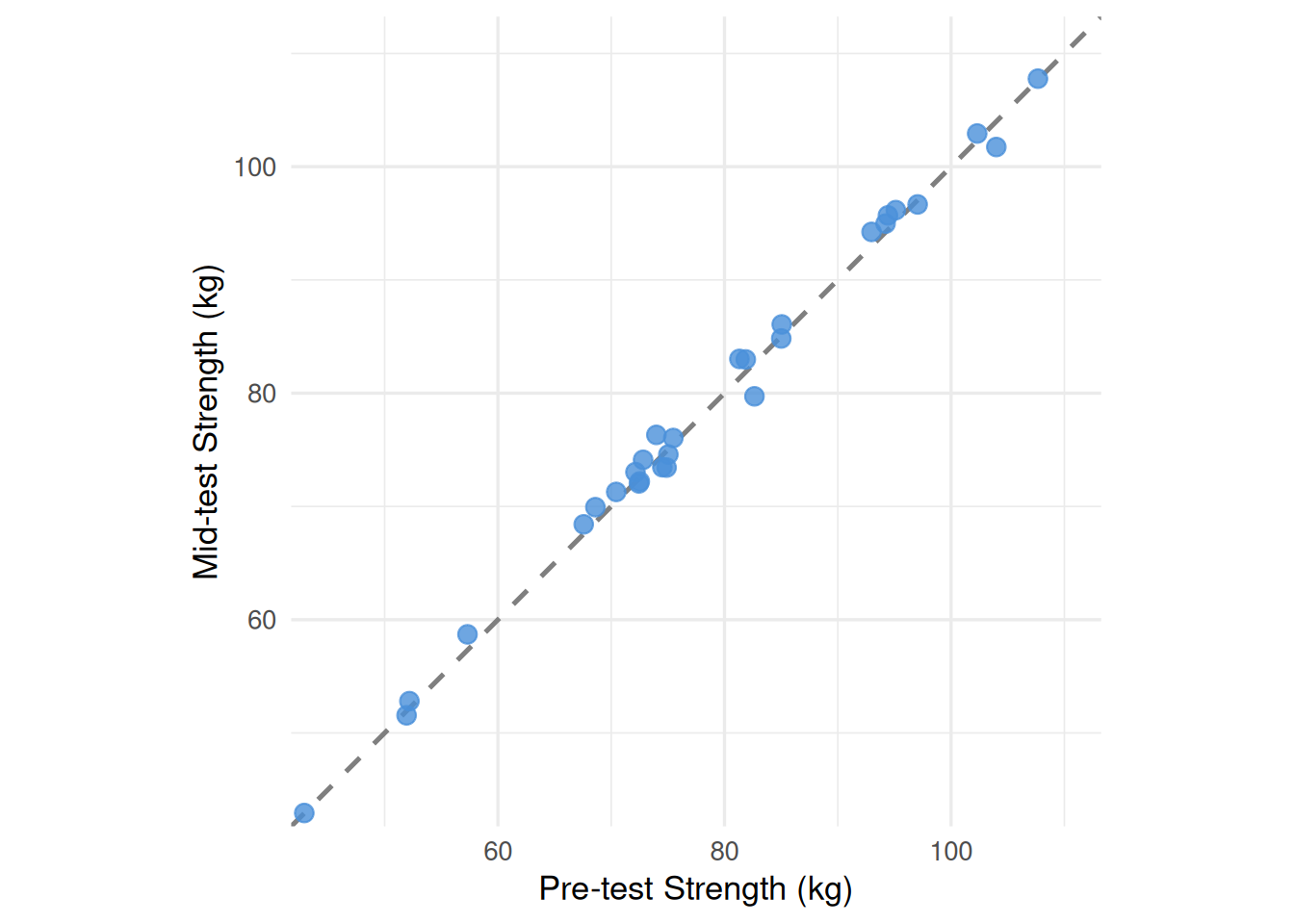
Both ICC values are in the excellent range^[6]. The near-identical consistency and absolute agreement values indicate negligible systematic bias between occasions — the dynamometer assessment produces virtually the same scores at both time points, with the small difference being random rather than directional. Figure 18.1 confirms this visually.

library(ggplot2)
library(dplyr)

set.seed(42)

n <- 30
pre  <- rnorm(n, mean = 76.34, sd = 13.70)
mid  <- pre + rnorm(n, mean = 0.52, sd = 1.15)

df_icc <- data.frame(pre = pre, mid = mid)

ggplot(df_icc, aes(x = pre, y = mid)) +
  geom_abline(slope = 1, intercept = 0, linetype = "dashed",
              color = "grey50", linewidth = 0.9) +
  geom_point(color = "#4A90D9", size = 3, alpha = 0.8) +
  labs(x = "Pre-test Strength (kg)", y = "Mid-test Strength (kg)") +
  coord_fixed(ratio = 1, xlim = c(45, 110), ylim = c(45, 110)) +
  theme_minimal(base_size = 13)

Figure 18.1: Test-retest scatter plot for strength_kg (control group, n = 30). Each point represents one participant’s pre-test (x-axis) and mid-test (y-axis) strength. Points falling on the dashed diagonal identity line indicate perfect agreement between occasions. The tight clustering around the diagonal reflects the excellent ICC(2,1) = .997.

18.7 Standard Error of Measurement

18.7.1 What SEM represents

The ICC tells us how much of the score variance is signal versus noise, but it does so in relative terms — as a proportion. Researchers and clinicians often need to understand reliability in the original units of measurement: by how many kilograms or seconds might a single measurement deviate from a participant’s true value? The Standard Error of Measurement (SEM) provides this answer.

The SEM is the standard deviation of repeated measurements on the same individual under identical conditions — the spread of scores that would be obtained if a person were tested infinitely many times with no learning, fatigue, or change in true ability. In practice, it is estimated from a reliability study:

\[\text{SEM} = SD_{\text{pooled}} \times \sqrt{1 - \text{ICC}}\]

where \(SD_{\text{pooled}}\) is the pooled standard deviation across both test occasions and ICC is the single-measures value^[4]. Note the key implication: SEM depends on both the variability of the sample (SD) and the reliability (ICC). A test can have a high ICC but a large SEM if the sample is highly variable; conversely, a modest ICC can produce a small SEM in a homogeneous sample. Both statistics should always be reported together.

18.7.2 Worked example: SEM for three variables

Using ICC(2,1) consistency values and the pooled SDs from the core_session.csv control group test-retest data:

Table 18.2: SEM for three performance variables from the core_session.csv test-retest dataset.

Variable	Pooled SD	ICC	SEM	Interpretation
strength_kg	13.49 kg	.997	0.82 kg	Typical measurement error ≈ 0.82 kg
vo2_mlkgmin	7.06 mL·kg⁻¹·min⁻¹	.922	1.97 mL·kg⁻¹·min⁻¹	Typical error ≈ 2 mL·kg⁻¹·min⁻¹
sprint_20m_s	0.38 s	.832	0.14 s	Typical error ≈ 0.14 s

The SEM for strength_kg (0.82 kg) is remarkably small relative to the group mean (≈ 77 kg), reflecting the excellent reliability of the dynamometer protocol. The SEM for vo2_mlkgmin (1.97 mL·kg⁻¹·min⁻¹) is larger in absolute terms and reflects the additional sources of variability in maximal aerobic testing (motivation, pacing, environmental factors). The sprint test SEM (0.14 s) appears small but must be evaluated against the range of sprint times in the group (approximately 3.3–4.5 s) and the magnitudes of change expected from training.

WarningCommon mistake: Confusing SEM with the standard error of the mean

The SEM in reliability analysis — Standard Error of Measurement — is completely different from the standard error of the mean (SE) introduced in Chapter 8. The SE of the mean describes uncertainty about a group average; it equals SD / √n and decreases as sample size grows. The SEM in reliability describes uncertainty about individual scores; it reflects measurement precision and does not depend on sample size in the same way. The abbreviation “SEM” is unfortunately used for both in the literature — always verify from context which one is intended.

18.8 Minimal Detectable Change

18.8.1 From SEM to individual change detection

The SEM tells us the expected spread of scores around a participant’s true value. To determine whether an observed change in an individual participant represents genuine improvement or merely measurement noise, we extend the SEM logic to the difference score between two occasions. Because differences between two independent measurements each carry their own error, the SD of a difference score is \(\text{SEM} \times \sqrt{2}\). Multiplying by 1.96 creates a 95% interval around a change of zero:

\[\text{MDC}_{95} = \text{SEM} \times 1.96 \times \sqrt{2}\]

The MDC₉₅ is the smallest change that can be detected with 95% confidence as exceeding the limits of measurement error alone^[2,4]. A change smaller than MDC₉₅ could plausibly have occurred by chance even if the participant’s true score did not change at all; a change exceeding MDC₉₅ is unlikely to be explained by measurement noise.

18.8.2 Worked example: MDC₉₅ for all three variables

Table 18.3: MDC₉₅ values for three performance variables.

Variable	SEM	MDC₉₅	Practical meaning
strength_kg	0.82 kg	2.26 kg	A gain of < 2.26 kg might just be noise
vo2_mlkgmin	1.97 mL·kg⁻¹·min⁻¹	5.45 mL·kg⁻¹·min⁻¹	Need > 5.45 mL·kg⁻¹·min⁻¹ gain to be confident it’s real
sprint_20m_s	0.14 s	0.40 s	Speed improvement must exceed 0.40 s to be reliable

Recall from Chapter 15 that the training group’s mean strength gain from pre- to post-test was 5.39 kg. With MDC₉₅ = 2.26 kg, this group-level change comfortably exceeds the threshold of detectable change. At the individual level, a participant who improved from 75 kg to 78 kg (a change of 3 kg) would just exceed the MDC₉₅, suggesting a real — though modest — improvement. A participant who improved from 80 kg to 81.5 kg (a change of 1.5 kg) would fall below it; that improvement cannot be distinguished from measurement noise.

18.9 Bland-Altman method

18.9.1 Limits of agreement

The Bland-Altman method^[7] is a graphical and numerical complement to the ICC. Rather than summarizing reliability as a single correlation, it plots each participant’s mean of the two measurements (x-axis) against their difference between the two measurements (y-axis). This layout makes two important features immediately visible: (1) the bias — any systematic tendency for one occasion to score higher than the other, estimated as the mean of all difference scores; and (2) the limits of agreement — the interval within which 95% of individual differences are expected to fall:

\[\text{LoA} = \bar{d} \pm 1.96 \times SD_d\]

where \(\bar{d}\) is the mean difference (bias) and \(SD_d\) is the standard deviation of the differences^[1,7].

The limits of agreement answer the clinically practical question: “If I measure the same person twice, how far apart might the two readings be?” They translate reliability into measurement units that practitioners can directly compare against the smallest clinically important difference for the variable of interest.

18.9.2 Interpreting the Bland-Altman plot

Two features of the plot require particular attention beyond the bias and limits:

Heteroscedasticity: If the spread of the differences increases as the mean score increases (the plot fans out to the right), the measurement error is proportional to the magnitude of the score rather than constant. This pattern is common in variables that span a large range (e.g., jump height across elite and recreational athletes). When heteroscedasticity is present, log-transforming the data before computing Bland-Altman statistics produces more interpretable limits of agreement.

Systematic bias: A non-zero mean difference (bias) that departs significantly from zero indicates that one measurement occasion consistently produces higher or lower values than the other. Common causes include a learning effect on the second test occasion, assessor drift over time, or equipment recalibration between sessions. The paired t-test on the difference scores tests whether bias differs significantly from zero.

18.9.3 Worked example: Bland-Altman for strength

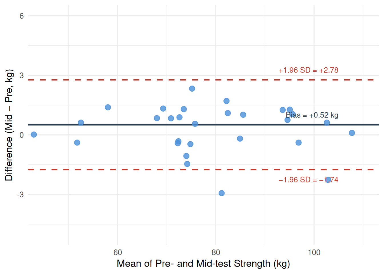
Figure 18.2 shows the Bland-Altman plot for strength_kg (control group, pre vs. mid). The mean difference (bias) is 0.52 kg — mid-test scores were on average 0.52 kg higher than pre-test scores, a small but detectable upward drift that may reflect a modest familiarization or practice effect over the first measurement block. The limits of agreement are −1.74 to 2.78 kg: 95% of individuals’ test-retest differences fall within this window. There is no obvious heteroscedasticity; the spread of differences is roughly constant across the range of strength values.

library(ggplot2)
library(dplyr)

set.seed(42)

n <- 30
pre <- rnorm(n, mean = 76.34, sd = 13.70)
mid <- pre + rnorm(n, mean = 0.517, sd = 1.153)

df_ba <- data.frame(
  avg  = (pre + mid) / 2,
  diff = mid - pre
)

bias     <-  0.517
loa_up   <-  2.777
loa_down <- -1.743

ggplot(df_ba, aes(x = avg, y = diff)) +
  geom_hline(yintercept = bias,     color = "#2C3E50", linewidth = 1.0) +
  geom_hline(yintercept = loa_up,   color = "#C0392B", linewidth = 0.9,
             linetype = "dashed") +
  geom_hline(yintercept = loa_down, color = "#C0392B", linewidth = 0.9,
             linetype = "dashed") +
  geom_point(color = "#4A90D9", size = 3, alpha = 0.8) +
  annotate("text", x = 105, y = bias + 0.5,
           label = "Bias = +0.52 kg", hjust = 1, size = 3.5, color = "#2C3E50") +
  annotate("text", x = 105, y = loa_up + 0.5,
           label = "+1.96 SD = +2.78", hjust = 1, size = 3.5, color = "#C0392B") +
  annotate("text", x = 105, y = loa_down - 0.5,
           label = "−1.96 SD = −1.74", hjust = 1, size = 3.5, color = "#C0392B") +
  labs(x = "Mean of Pre- and Mid-test Strength (kg)",
       y = "Difference (Mid − Pre, kg)") +
  coord_cartesian(xlim = c(45, 110), ylim = c(-5, 6)) +
  theme_minimal(base_size = 13)

Figure 18.2: Bland-Altman plot for strength_kg test-retest reliability (control group, n = 30). Each point shows one participant’s mean strength (x-axis) versus the difference between mid-test and pre-test strength (y-axis). The solid horizontal line is the mean difference (bias = +0.52 kg); the dashed lines are the 95% limits of agreement (−1.74 to +2.78 kg).

18.10 Comparing reliability across variables

The three variables in Table 18.2 and Table 18.3 illustrate how reliability varies substantially across measurement tools, even within the same sample and protocol. strength_kg shows near-perfect reliability (ICC = .997), reflecting the precision of a standardized dynamometer protocol and the low biological day-to-day variability of isometric strength in rested participants. vo2_mlkgmin shows good but lower reliability (ICC = .922), consistent with the known variability of maximal aerobic tests — participants must achieve a true maximal effort on each occasion, and small differences in motivation or pacing produce meaningful score fluctuations. sprint_20m_s sits between the two (ICC = .832), reflecting the combined noise of timing equipment precision, reaction time variability, and subtle lane condition differences.

These differences have direct consequences for the statistical analyses in previous chapters. The ANCOVA in Chapter 17 exploited a pre-post correlation of r = .980 for strength — a correlation that could not be that high unless the measurement itself were highly reliable. Had the dynamometer reliability been ICC = .70 (good but not excellent), the pre-post correlation would have been attenuated downward and the precision gain from ANCOVA would have been substantially smaller. This attenuation phenomenon is systematic: the observed correlation between any two variables can never exceed the geometric mean of their individual reliabilities — a principle known as disattenuation^[1].

18.11 Factors affecting reliability

Several modifiable factors influence the reliability of movement science measurements, and understanding them guides both study design and protocol standardization.

Biological variability is the irreducible day-to-day fluctuation in a participant’s true physiological state — driven by sleep, nutrition, hydration, circadian rhythms, and accumulated fatigue. Reliability studies conducted over longer intervals (days to weeks) will generally yield lower ICC values than those conducted within a single session, because more biological variation is captured in the difference score. Researchers should report the inter-session interval used in their reliability study.

Protocol standardization is perhaps the most controllable source of variability. Detailed, written protocols that specify warm-up duration, rest intervals, equipment settings, verbal instructions, and scoring rules reduce assessor-to-assessor and session-to-session inconsistency. Equipment calibration before each testing session eliminates systematic drift.

Participant familiarity affects reliability in tasks with a motor learning component. Novice participants may show meaningful performance improvements between test sessions simply due to practice, not genuine physiological change — a confound that manifests as systematic bias in the Bland-Altman analysis. Including a familiarization session before the first reliability measurement is strongly recommended for novel assessment tasks^[1,8].

Rater training matters substantially for subjective or semi-objective assessments (movement quality scores, pain ratings, clinical examination findings). Assessors should be trained to criterion on pilot data before the study begins, with inter-rater reliability verified and reported as a separate analysis from test-retest reliability.

18.12 Reliability and statistical power

Poor reliability has a direct, quantifiable cost in statistical power. If the true correlation between two variables is \(\rho\), the observed (attenuated) correlation in data with measurement reliabilities \(r_{xx}\) and \(r_{yy}\) is:

\[r_{\text{observed}} = \rho \cdot \sqrt{r_{xx} \cdot r_{yy}}\]

Even with a true correlation of \(\rho = .70\), if both variables are measured with reliability of .80, the observed correlation will be only \(.70 \times \sqrt{.80 \times .80} = .70 \times .80 = .56\) — a meaningful underestimate that inflates the required sample size. For analysis of variance and t-tests, poor reliability inflates the within-group error variance (MS_error), directly reducing the F-ratio. A 10-point improvement in ICC (from .80 to .90) can meaningfully reduce the required sample size by 20–30% for the same statistical power^[4,9].

This connection explains why a full description of measurement reliability is not an optional add-on to a methods section but a core requirement. Readers cannot evaluate the plausibility of null findings — or trust the effect size estimates behind positive findings — without knowing how much noise was present in the measurements that generated them.

18.13 Reporting reliability in APA style

18.13.1 Template

Test-retest reliability was assessed using ICC(2,1) absolute agreement (single measures) following the guidelines of^[6]. [Variable] demonstrated [classification] reliability (ICC = [value], 95% CI [lower, upper]). The SEM was [value] [units] and the MDC₉₅ was [value] [units], indicating that individual changes of at least [MDC₉₅ value] are required to exceed the limits of measurement error with 95% confidence. Bland-Altman analysis indicated a mean bias of [value] [units] (mid − pre), with 95% limits of agreement from [lower LoA] to [upper LoA] [units].

18.13.2 Full APA example

Test-retest reliability of the isometric dynamometer strength assessment was evaluated using the control group (n = 30) across two measurement occasions separated by six weeks. ICC(2,1) absolute agreement (single measures) was computed following^[6]. Strength (strength_kg) demonstrated excellent reliability, ICC(2,1) = .996 (95% CI [.993, .998]). The SEM was 0.82 kg and the MDC₉₅ was 2.26 kg, indicating that individual strength changes must exceed 2.26 kg to be confidently attributed to genuine change rather than measurement error. Bland-Altman analysis revealed a small mean bias of +0.52 kg (mid > pre), with 95% limits of agreement of −1.74 to +2.78 kg. No evidence of heteroscedasticity was observed. Aerobic capacity (vo2_mlkgmin) demonstrated good reliability, ICC(2,1) = .919 (95% CI [.841, .959]), with SEM = 1.97 mL·kg⁻¹·min⁻¹ and MDC₉₅ = 5.45 mL·kg⁻¹·min⁻¹.

18.14 Common pitfalls and best practices

18.14.1 Pitfall 1: Using Pearson r instead of ICC

The Pearson correlation coefficient measures the linear association between two variables but is insensitive to systematic bias between test occasions. Two instruments can produce scores with r = .99 while one consistently reads 10 units higher than the other — the Pearson r would be unchanged. ICC(2,1) absolute agreement captures both the correlation and the systematic offset, making it the appropriate choice for test-retest reliability^[4,5]. Never substitute Pearson r for ICC in a reliability analysis.

18.14.2 Pitfall 2: Reporting ICC without confidence intervals

A single ICC point estimate conveys no information about precision. An ICC of .87 computed from n = 10 participants has a 95% CI of approximately [.57, .97] — spanning the range from “moderate” to “excellent.” The same ICC from n = 50 participants yields a CI of approximately [.79, .92] — a much tighter and more interpretable estimate. Minimum sample size recommendations for reliability studies typically range from n = 30 to n = 50 to obtain reasonably narrow confidence intervals^[4,6].

18.14.3 Pitfall 3: Ignoring systematic bias

A high ICC and a narrow SEM do not guarantee the absence of systematic bias. A protocol that consistently produces higher scores on the second test occasion (due to learning) can still have ICC = .99 — because participants maintain their rank ordering perfectly, even though everyone scores slightly higher the second time. Systematic bias is invisible to ICC but visible in the Bland-Altman mean difference and detectable with a paired t-test on the difference scores. Always pair ICC with Bland-Altman analysis.

18.14.4 Pitfall 4: Applying group-level MDC₉₅ to individual decisions without caution

The MDC₉₅ is computed from group data and represents the typical boundary of measurement error across the sample. Individual participants may have more or less measurement variability than the group average. In clinical practice, the MDC₉₅ is a useful starting point for individual change interpretation, but it should be supplemented by clinical judgment and, when available, the Minimal Clinically Important Difference (MCID) — the smallest change perceived as meaningful by the patient or client^[2].

18.15 Chapter summary

Reliability is the statistical foundation beneath every analysis in this textbook. Without it, observed differences between groups may be artifacts of measurement noise rather than genuine treatment effects; observed correlations will be attenuated below their true magnitudes; and conclusions about individual improvement will be unreliable. The four tools introduced in this chapter — ICC, SEM, MDC₉₅, and Bland-Altman analysis — provide complementary perspectives on measurement precision, each answering a different question about how much trust can be placed in a set of scores^[1,4,7].

The worked examples using core_session.csv demonstrated that the dynamometer strength assessment used throughout this textbook has excellent test-retest reliability (ICC(2,1) = .997), with a SEM of 0.82 kg and MDC₉₅ of 2.26 kg. These values justify the high statistical power and precise estimates obtained in the ANCOVA and repeated measures analyses of earlier chapters — strong statistical results require strong measurements. The VO₂max and sprint assessments showed good but lower reliability, consistent with the greater biological and motivational variability inherent in maximal aerobic and speed testing. Chapter 19 continues the journey beyond the normal distribution, introducing nonparametric methods for situations where distributional assumptions cannot be justified — the statistical toolkit for data that resists the parametric framework that has guided the analyses up to this point.

18.16 Key terms

reliability; validity; systematic error; random error; intraclass correlation coefficient (ICC); ICC(2,1); ICC(3,1); absolute agreement; consistency; single measures; average measures; Standard Error of Measurement (SEM); Minimal Detectable Change (MDC₉₅); Bland-Altman method; limits of agreement; bias; heteroscedasticity; disattenuation; test-retest reliability; inter-rater reliability

18.17 Practice: quick checks

Pearson r measures the strength and direction of the linear association between two sets of scores, but it is insensitive to systematic differences in level between occasions. Two instruments whose scores are related by the equation Y = X + 10 (one always reads 10 units higher) will produce r = 1.00, suggesting perfect reliability — when in fact there is a substantial and consistent bias. ICC(2,1) absolute agreement accounts for both the correlation and any mean-level difference between occasions. If the means differ systematically, the absolute agreement ICC will be lower than the consistency ICC, flagging the problem. In reliability research, the goal is to detect all forms of measurement inconsistency, not just rank-order inconsistency, making ICC the appropriate tool.

The ICC of .91 is “excellent” by^[6] benchmarks, which is reassuring. However, ICC alone is not sufficient for individual decision-making — the SEM and MDC₉₅ are also essential. If the sample SD for jump height is 8 cm, then SEM = 8 × √(1 − .91) = 8 × .30 = 2.4 cm, and MDC₉₅ = 2.4 × 1.96 × √2 = 6.65 cm. This means the coach cannot confidently conclude that an athlete has genuinely improved unless their jump height increases by at least 6.65 cm between assessments. Whether that threshold is acceptable depends on the expected magnitude of training-induced change. An intervention that typically improves jump height by 2–3 cm would be undetectable against this noise floor despite the excellent ICC.

The positive bias of +3 cm indicates that the second measurement occasion consistently produces scores 3 cm higher than the first — a systematic upward drift that could reflect a learning effect, assessor drift, or equipment recalibration. The limits of agreement (−2 to +8 cm) show that 95% of individuals’ test-retest differences fall within this window: while most participants score higher on occasion 2, a few score slightly lower (down to −2 cm), and some score considerably higher (up to +8 cm above their occasion 1 value). The asymmetric limits (the upper bound is further from bias than the lower) suggest the systematic bias combines with random variability in a way that produces more large positive differences than large negative ones. A paired t-test on the differences would likely confirm the bias is statistically significant, and a familiarization session before the first test occasion should be added to future protocols.

The MDC₉₅ = 3.2 × 1.96 × √2 = 8.88 errors. The patient’s observed improvement (5 errors) falls below the MDC₉₅, meaning this change could plausibly have occurred through measurement noise alone — with 95% confidence, we cannot rule out that the true change was zero. This is not the same as saying the patient did not improve; it means the measurement instrument is not precise enough to confirm that they did. Two responses are appropriate: (1) note the finding honestly in clinical records, acknowledging measurement uncertainty; and (2) consider whether additional assessments, a more reliable instrument, or a longer follow-up might produce a more conclusive picture. The MDC₉₅ should be computed and reported before a study begins, so that sample sizes and expected effect sizes can be planned accordingly.

Poor reliability inflates the within-group variance in the outcome, which directly increases MS_error — the denominator of the F-ratio. A larger MS_error means a smaller F for the same group mean difference, reducing statistical power and increasing the probability of a Type II error (failing to detect a real group difference). Quantitatively, if ICC = .80, then 20% of each observed score is measurement noise, and that noise accumulates in the within-group variance. Effect sizes (η²_p, Cohen’s d) are also attenuated: the observed effect between groups will be smaller than the true effect because measurement error spreads the score distributions. This is why establishing strong measurement reliability before the main study — and reporting it in the methods section — is not merely a procedural formality but a direct contributor to the study’s ability to detect true effects.

In tasks with a significant motor learning component — novel movement patterns, unfamiliar equipment, or assessments requiring maximal effort — participants typically improve their performance between the first and second exposure simply through practice, not genuine physiological change. If the first test occasion is the “pre-test” and the second is the “post-test” in a reliability study, this learning effect creates systematic positive bias: scores are consistently higher on occasion 2. This inflates the mean difference in the Bland-Altman analysis and, depending on the design, can artificially inflate the ICC if learning is uniform across participants (everyone improves by roughly the same amount, maintaining rank order) or deflate it if learning is variable (some participants improve more than others, disrupting rank order). Adding one or two familiarization sessions before data collection allows participants to reach a performance plateau, after which genuine test-retest differences reflect measurement precision rather than learning.

NoteRead further

^[1] remains the most comprehensive introduction to reliability methodology for sport and exercise scientists.^[4] provides a practical guide to selecting and computing ICC and SEM with worked examples.^[6] is the standard reference for ICC model selection and interpretation benchmarks.^[7] is the original and most-cited presentation of the limits of agreement method.^[2] covers reliability within a broader clinical research methods context and is especially useful for rehabilitation and applied settings.

NoteNext chapter

Chapter 19 introduces Nonparametric Statistics — methods that do not require the normality assumption underpinning the t-tests, ANOVAs, and regression procedures in earlier chapters. You will learn when and why to use rank-based alternatives such as the Mann-Whitney U test, Kruskal-Wallis ANOVA, Wilcoxon signed-rank test, and Friedman’s test, and how to quantify effect sizes in nonparametric settings.

1. Atkinson, G., & Nevill, A. M. (1998). Statistical methods for assessing measurement error (reliability) in variables relevant to sports medicine. Sports Medicine, 26(4), 217–238. https://doi.org/10.2165/00007256-199826040-00002

2. Portney, L. G., & Watkins, M. P. (2020). Foundations of clinical research: Applications to practice.

3. Thomas, L. (2015). How to estimate power and sample size. Trauma Surgery & Acute Care Open, 1(1), e000005. https://doi.org/10.1136/tsaco-2015-000005

4. Weir, J. P. (2005). Quantifying test-retest reliability using the intraclass correlation coefficient and the SEM. Journal of Strength and Conditioning Research, 19(1), 231–240. https://doi.org/10.1519/15184.1

5. Shrout, P. E., & Fleiss, J. L. (1979). Intraclass correlations: Uses in assessing rater reliability. Psychological Bulletin, 86(2), 420–428. https://doi.org/10.1037/0033-2909.86.2.420

6. Koo, T. K., & Li, M. Y. (2016). A guideline of selecting and reporting intraclass correlation coefficients for reliability research. Journal of Chiropractic Medicine, 15(2), 155–163. https://doi.org/10.1016/j.jcm.2016.02.012

7. Bland, J. M., & Altman, D. G. (1986). Statistical methods for assessing agreement between two methods of clinical measurement. Lancet, 327(8476), 307–310. https://doi.org/10.1016/S0140-6736(86)90837-8

8. Hopkins, W. G. (2000). Measures of reliability in sports medicine and science. Sports Medicine, 30(1), 1–15. https://doi.org/10.2165/00007256-200030010-00001

9. Cohen, J. (1988). Statistical power analysis for the behavioral sciences (2nd ed.). Lawrence Erlbaum Associates.