This blog post explores Factorial Analysis of Variance (ANOVA) in a between-within design, covering key assumptions, equations, and calculations. Readers will learn about effect size measures, post-hoc analysis options, and non-parametric alternatives. The post also provides steps to perform Factorial ANOVA using popular statistical software packages like jamovi, SPSS, and R Studio, and guidance on reporting results in APA style, enabling readers to effectively apply this statistical method in real-world research settings.
Understand the basic principles and assumptions of within-within factorial ANOVA.
Understand how to design and conduct a within-within factorial ANOVA study.
Understand how to interpret the results of a within-within factorial ANOVA, including main effects and interactions.
Understand how to conduct post-hoc tests to compare levels of the within-subjects factor.
Understand how to address violations of the assumptions of within-within factorial ANOVA, such as non-normality of the data.
Understand the non-parametric alternatives to within-within factorial ANOVA, such as the Friedman test.
Understand how to run a within-within factorial ANOVA and LMM in popular statistical software such as SPSS and Jamovi.
Understand how to select appropriate models and methods based on the specific research question and data.
1 Decision
List of questions that a researcher may need to consider when deciding to use a Mixed Factorial ANOVA:
Is there at least one between-subjects factor and one within-subjects factor? If not, then a mixed factorial ANOVA is not appropriate.
Is the dependent variable continuous? If not, then a mixed factorial ANOVA is not appropriate.
Are the independent variables dependent or related to each other? If yes, then a mixed factorial ANOVA may be appropriate.
Are the data normally distributed? If the data are not normally distributed, then the researcher may consider using a nonparametric alternative or transforming the data to meet the normality assumption.
Are the variances equal across groups? If not, then the researcher may consider using Welch’s ANOVA or a mixed design Welch’s ANOVA.
Are there any significant interactions between the between-subjects and within-subjects factors? If yes, then the researcher should interpret and report these interactions.
Are there any significant main effects of the between-subjects or within-subjects factors? If yes, then the researcher should interpret and report these main effects.
Are there any significant simple effects or post-hoc comparisons? If yes, then the researcher should conduct and interpret these tests to further explore the effects of the independent variables on the dependent variable.
Note
The website StatKat has several tools to help with this decision.
This dataset consists of 30 participants who have undergone balance and strength training interventions. The dataset contains the following variables:
ID: A unique identifier for each participant.
Pretest_Balance: The Functional Reach Test (FRT) score for balance at the beginning of the intervention (pretest).
Midtest_Balance: The FRT score for balance at the midpoint of the intervention (midtest).
Posttest_Balance: The FRT score for balance at the end of the intervention (posttest).
Pretest_Strength: The strength score at the beginning of the intervention (pretest).
Midtest_Strength: The strength score at the midpoint of the intervention (midtest).
Posttest_Strength: The strength score at the end of the intervention (posttest).
Gender: The gender of each participant (Male or Female).
The dataset includes information on participants’ motor performance in terms of balance (FRT scores) and strength over three time points (pretest, midtest, and posttest) and their gender. This dataset can be used to investigate the effectiveness of balance and strength training interventions on motor performance over time and any potential differences in outcomes based on gender.
A lower FRT score suggests poorer balance and stability, which may be associated with a higher risk of falling. In contrast, a higher FRT score indicates better balance and stability, suggesting a lower risk of falling. By examining the effects of time and training type on FRT scores, this study aims to determine whether balance and strength training interventions can improve motor performance and, by extension, reduce the risk of falling among the participants.
3 Intro to Mixed \(f\)ANOVA
Kinesiology research often involves studying the effects of multiple independent variables on a continuous dependent variable. To analyze these complex relationships, researchers commonly use statistical methods such as ANOVA. Within-subjects and between-subjects ANOVA are two common approaches for analyzing the effects of independent variables on a dependent variable. However, there are situations where a combination of both approaches, called mixed factorial ANOVA, may be appropriate. Mixed factorial ANOVA allows researchers to examine the effects of both within-subjects and between-subjects factors on a continuous dependent variable, as well as any potential interactions between these factors.
In this blog post, we will explore the basics of mixed factorial ANOVA, including when it is appropriate to use, how to conduct the analysis, and how to interpret the results. We will also provide real-world examples from the field of kinesiology to demonstrate how mixed factorial ANOVA can be used to answer research questions and improve our understanding of complex relationships between independent and dependent variables.
4 Assumptions
Normality: The dependent variable should be normally distributed within each group defined by the combination of the independent variables. This assumption can be checked using normal probability plots or statistical tests such as the Shapiro-Wilk test.
Homogeneity of variance: The variances of the dependent variable should be equal across groups defined by the combination of the independent variables. This assumption can be checked using statistical tests such as Levene’s or Brown-Forsythe’s.
Sphericity: The variances of the differences between all pairs of levels of the within-subjects factor should be equal. This assumption is referred to as sphericity and is important because violations of sphericity can lead to inflated Type I error rates. This assumption can be checked using statistical tests such as Mauchly’s or Greenhouse-Geisser’s correction.
Independence: Observations within each group defined by the combination of the independent variables should be independent.
It is important to note that violation of these assumptions can affect the validity of the mixed factorial ANOVA analysis results. If these assumptions are not met, the researcher may consider using alternative statistical methods, such as non-parametric tests or data transformations, or correcting for violations through various means, such as using the Greenhouse-Geisser correction for violations of sphericity. Checking these assumptions should be a standard part of any mixed factorial ANOVA analysis, as it helps to ensure that the results are valid and reliable.
5 Equations
Equations needed for hand calculation of mixed factorial ANOVA:
where \(a\) is the number of levels for the between-subjects factor, \(b\) is the number of levels for the within-subjects factor, and \(n\) is the number of observations per cell.
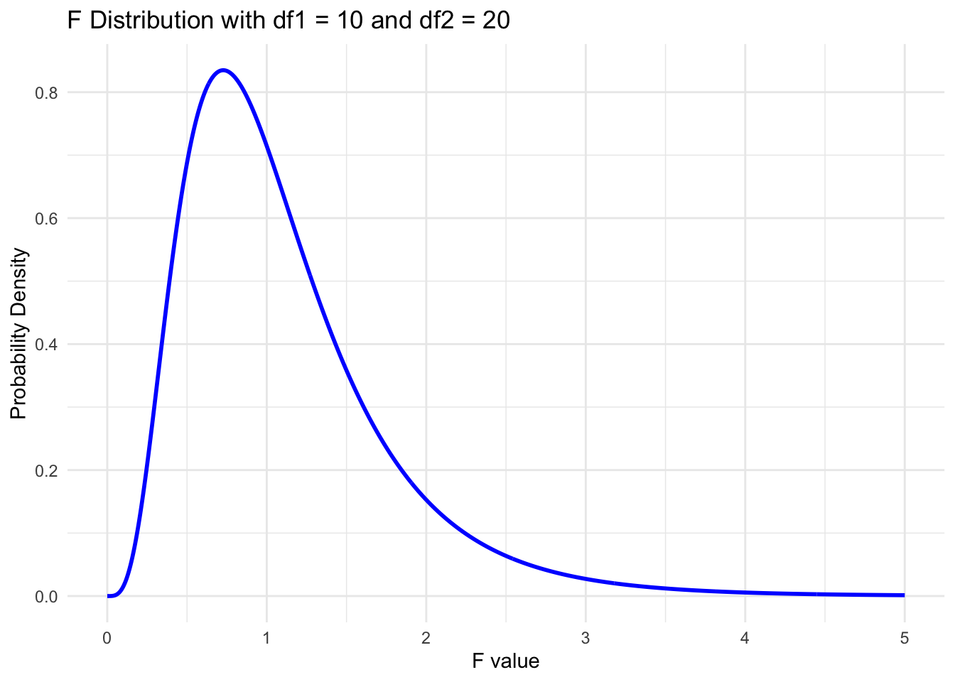
6 F Distribution
The F distribution[1], also known as the Fisher-Snedecor distribution, is a continuous probability distribution that is widely used in statistical hypothesis testing, particularly in the analysis of variance (ANOVA). It is named after Ronald A. Fisher and George W. Snedecor, two prominent statisticians who contributed significantly to its development.
The F-distribution used in the Between-Between Factorial ANOVA is the same as that used in One-Way ANOVA. The F-distribution is a continuous probability distribution that arises frequently as the null distribution of the test statistic in ANOVA, regardless of whether it is a One-Way or Factorial ANOVA.
However, the degrees of freedom for the F-distribution will differ between One-Way ANOVA and Factorial ANOVA. In One-Way ANOVA, the degrees of freedom are associated with the number of levels of a single independent variable.
In Factorial ANOVA, the degrees of freedom are associated with the number of levels of multiple independent variables and their interactions. When comparing F-ratios to critical F-values, you need to consider the appropriate degrees of freedom for your specific test. In both One-Way and Factorial ANOVA, you look up the critical F-value in an F-distribution table based on the numerator and denominator degrees of freedom and the chosen significance level (usually α = 0.05). If the calculated F-ratio is greater than the critical F-value, you can reject the null hypothesis and conclude that there is a significant effect.
Some key characteristics of the F distribution are:
It is always non-negative, as it represents the ratio of two chi-square distributions.
It is asymmetric and positively skewed, with a longer tail on the right side.
The peak of the distribution shifts to the right as the degrees of freedom increase.
As both degrees of freedom approach infinity, the F distribution converges to a normal distribution.
suppressMessages(pacman::p_load("ggplot2", "ggthemes"))# Set the parameters for the F distributiondf1 <-10# degrees of freedom for the numeratordf2 <-20# degrees of freedom for the denominator# Create a function to calculate the probability density function (pdf) of the F distributionf_pdf <-function(x) {df(x, df1, df2)}# Define the range of x values to plotx_range <-seq(0, 5, length.out =1000)# Plot the F distribution using ggplot2suppressWarnings(ggplot(data.frame(x = x_range, y =f_pdf(x_range)), aes(x = x, y = y)) +geom_line(color ="blue", size =1) +ggtitle(paste("F Distribution with df1 =", df1, "and df2 =", df2)) +xlab("F value") +ylab("Probability Density") +theme_minimal())
7 Measure of effect size
Measures of effect size for mixed factorial ANOVA can help researchers interpret the magnitude of the effects found in their analysis. Here are two commonly used measures of effect size for mixed factorial ANOVA:
Partial eta-squared (\(\eta_{p}^{2}\)): This measure of effect size represents the proportion of variance in the dependent variable accounted for by a specific independent variable or interaction while controlling for other independent variables. It is calculated by dividing the sum of squares for an effect by the sum of squares total. For example, the partial eta-squared for the between-subjects factor A would be calculated by dividing the sum of squares for factor A by the sum of squares total. A commonly used rule of thumb is that a partial eta-squared value of 0.01 represents a small effect, 0.06 represents a medium effect, and 0.14 represents a large effect.
Cohen’s d: This measure of effect size represents the standardized mean difference between two groups. In the context of mixed factorial ANOVA, Cohen’s d can be used to calculate the effect size for a specific contrast between levels of the independent variables. It is calculated by dividing the difference in means between two groups by the pooled standard deviation. A commonly used rule of thumb is that a Cohen’s d value of 0.2 represents a small effect, 0.5 represents a medium effect, and 0.8 represents a large effect.
By reporting measures of effect size, researchers can provide additional information about the magnitude of the effects found in their analysis, which can help interpret the practical significance of the results.
8 Post-Hoc analysis
Post hoc analysis is a statistical procedure conducted after an ANOVA to compare individual group means to determine which groups are significantly different from each other. The term “post hoc” is Latin for “after this, therefore because of this,” meaning that it is conducted after the ANOVA to avoid making assumptions about which groups will differ before analyzing the data.
Post hoc tests are necessary when a significant effect is found in the ANOVA, indicating that at least one of the groups differs significantly from the others. The most common post hoc tests used in mixed factorial ANOVA are:
Tukey’s Honestly Significant Difference (HSD) test: This test compares all possible pairs of means to determine which pairs are significantly different from each other. It controls for Type I error rates but is inappropriate if the sample sizes are unequal.
Bonferroni correction: This test is a more conservative approach that controls the overall Type I error rate by adjusting the significance level for each comparison. It is appropriate for unequal sample sizes and is more stringent than Tukey’s HSD test.
Scheffé’s test: This is also conservative and controls for the family-wise error rate but is less powerful than Tukey’s HSD test and Bonferroni correction.
Sidak’s test: This test is similar to Bonferroni correction but is less conservative and more powerful. It is appropriate for unequal sample sizes.
Fisher’s Least Significant Difference (LSD) test compares the means of two groups at a time and is inappropriate for multiple comparisons.
The choice of post hoc test depends on the specific research question and the data characteristics, such as sample size and variability. By conducting post hoc tests, researchers can determine which specific group means are significantly different from each other, providing a more detailed understanding of the patterns of results in their data.
9 Result interpretation
Steps researchers would typically take to interpret the results of a mixed factorial ANOVA:
Check for violations of assumptions: Before interpreting the results of a mixed factorial ANOVA, researchers should check whether the assumptions of normality, homogeneity of variance, sphericity, and independence are met. If the assumptions are not met, the validity of the results may be compromised, and alternative statistical methods may need to be used.
Examine the main effects: Researchers should examine the main effects of the between-subjects factor(s) and within-subjects factor(s) to determine whether they are significant. A significant main effect indicates a significant difference between the means of the groups defined by that factor.
Examine the interaction effect: Researchers should examine the interaction effect to determine whether it is significant. A significant interaction effect indicates that the effect of one independent variable on the dependent variable differs depending on the level of the other independent variable.
Conduct post hoc tests: If there is a significant main effect or interaction effect, researchers may conduct post hoc tests to determine which specific group means are significantly different from each other.
Interpret effect sizes: Researchers should interpret effect sizes, such as partial eta-squared and Cohen’s d, to determine the practical significance of the results.
Consider the research question: Finally, researchers should consider the research question and the implications of the results. They should interpret the results in the context of the specific research question and the hypotheses being tested.
By following these steps, researchers can systematically and rigorously interpret the results of a mixed factorial ANOVA, providing a detailed understanding of the relationships between the independent and dependent variables in their study.
9.1 Interpreting Main Effects When Interaction is Significant
Interpreting the main effects becomes more complex when a significant interaction is present in a factorial ANOVA. A significant interaction suggests that the effect of one factor depends on the level of the other factor(s). In such cases, focusing on interpreting the interaction rather than the main effects alone is essential. Here is how to go about it:
Simple Effects Analysis: Conduct a simple effects analysis to disentangle the interaction. Simple effects analysis involves examining the effect of one factor at each level of the other factor(s). This helps identify specific combinations of factor levels contributing to the significant interaction.
Post Hoc Tests for Simple Effects: If a simple effect is significant, perform post hoc tests to identify which pairwise comparisons are significantly different. Use appropriate post hoc tests like Bonferroni, Tukey’s HSD, or Hochberg’s GT2, depending on your study design and sample sizes.
Graphical Representation: Plot the means of the dependent variable across the levels of one factor, with separate lines for each level of the other factor. This interaction plot will help visualize the nature of the interaction, making it easier to interpret the relationship between factors.
Interpretation: Describe the pattern observed in the interaction plot, paying attention to the differences in the slopes of the lines. Explain how the effect of one factor changes depending on the level of the other factor(s). It is crucial to interpret the main effects in the context of the interaction, as the main effects alone may not provide a complete picture of the relationships between variables.
Report the Results: Report the results of the interaction and the simple effects analysis, including any post hoc tests. Discuss the practical implications of these findings in relation to your research question.
Remember that the main effects should be interpreted with caution in the presence of a significant interaction. The interaction and the simple effects provide more meaningful insights into the relationships between the factors and the dependent variable.
10 Example
A researcher wanted to investigate the effects of gender on motor performance during balance training. Specifically, the study aimed to determine whether there were differences in motor performance between males and females during three-time points: pretest (T1), midtest (T2), and posttest (T3) of a balance training intervention. To conduct the study, 30 participants were recruited, 15 males and 15 females. All participants completed motor performance tests at three-time points during the balance training intervention. In addition, motor performance was assessed using the Functional Reach Test (FRT), which measures a participant’s ability to reach forward while maintaining balance.
The study design is a mixed factorial ANOVA, with the within-subjects factor of time (pretest, midtest, posttest) and the between-subjects factor of gender (male vs. female). The dependent variable is motor performance, measured by the FRT score during balance training.
The first step in interpreting the results would be to check for violations of assumptions, such as normality, homogeneity of variance, sphericity, and independence. If the assumptions are not met, appropriate transformations or nonparametric methods may need to be used.
The next step would be to examine the interaction effect of gender and time. This would determine whether the effect of gender on motor performance is dependent on the time points during balance training. If the interaction effect is significant, post hoc tests would be conducted to determine which specific group means are significantly different from each other.
The main effect of gender would also be examined to determine whether there are significant differences between the male and female groups during balance training. If the interaction effect is not significant, post hoc tests would be conducted to determine which specific group means are significantly different from each other.
Finally, the practical significance of the results would be interpreted by considering effect sizes, such as partial eta-squared and Cohen’s d, and the implications of the results for the research question would be discussed.
Using the provided dataset, a within-between factorial ANOVA could be conducted using statistical software to analyze the data.
10.1 Research question
The research question for this study is: “What are the effects of gender on motor performance during a balance training intervention, measured by the Functional Reach Test (FRT) score at three time points: pretest (T1), midtest (T2), and posttest (T3)?
10.2 Data set up
Table 1: Within-subjects ANOVA data setup
ID
Balance_T1
Balance_T2
Balance_T3
Gender
1
20
23
26
Male
2
25
28
31
Male
3
28
31
34
Male
4
22
24
27
Male
5
27
30
33
Male
10.3 Variables
The dependent variable is motor performance, measured by the Functional Reach Test (FRT) score.
The independent variables are gender (male vs. female) and time (pretest (T1), midtest (T2), and posttest (T3)).
Gender is a categorical variable, with two levels: male and female.
Time is a categorical variable, with three levels: pretest (T1), midtest (T2), and posttest (T3).
Motor performance is a continuous variable, measured by the FRT score.
This null hypothesis states that there is no significant difference in the means of motor performance across the three time points (pretest, midtest, and posttest) for both males and females combined (i.e., the means are equal).
This null hypothesis states that there is no significant difference in the means of motor performance between males and females combined across all time points (i.e., the means are equal).
\[
\textbf{Null Hypothesis (H0$_{TG}$):} \enspace \text{Absence of interaction}
\]
This null hypothesis states that there is no significant interaction effect between time and gender on motor performance.
This alternative hypothesis states that there is a significant difference in the means of motor performance across the three time points (pretest, midtest, and posttest) for both males and females combined (i.e., the means are not equal).
This alternative hypothesis states that there is a significant difference in the means of motor performance between males and females combined across all time points (i.e., the means are not equal).
\[
\textbf{Alternative Hypothesis (H1$_{TG}$):} \enspace \text{Presence of interaction}
\]
This alternative hypothesis states that there is a significant interaction effect between time and gender on motor performance.
10.5 Analyzing with jamovi
Jamovi is an open-source statistical software package that allows users to run various statistical analyses, including ANOVA (Analysis of Variance).
To perform a mixed factorial ANOVA in jamovi, you need one continuous variable for each within-subject measurement (e.g. pre/post), at least one grouping variable with at least two levels (e.g. treatment/control) and one variable to function as a between subject factor (e.g. gender). Here are the steps to follow:
In the box Repeated Measures Factors, write the name of your outcome variable (e.g. Time) and name the levels for each measurement occasion (e.g. Time 1, Time 2, Time 3).
Drag and drop your outcome variables to their respective cells in Repeated Measures Cells.
Move your grouping variable(s) to Between Subject Factors.
The result will be shown in the right panel.
Remember that the specific steps and options may change in newer versions of Jamovi, so be sure to consult the latest documentation and tutorials if you encounter any difficulties. The steps above refer to Version 2.3.21.0.
10.6 Analyzing with SPSS
To perform a mixed ANOVA in SPSS Statistics, you need to have groups that have been split on two “factors” (also known as independent variables), where one factor is a “within-subjects” factor and the other factor is a “between-subjects” factor. Here are the steps to follow:
Select Analyze from the list of menu options at the top of the screen.
Scroll down to General Linear Model and select Univariate.
In the Univariate window, select your dependent variable and your within-subjects and between-subjects factors.
The primary purpose of a mixed ANOVA is to understand if there is an interaction between these two factors on the dependent variable.
Note
The specific steps and options may vary depending on the version of SPSS you are using, as well as the specific details of your data and analysis. The steps above are for version 28.
SPSS Syntax
Here is the SPSS syntax for the 3x2 Between-Between Factorial ANOVA using your dataset:
Replace dependent_variable with the name of your dependent variable, within_subject_factor1 and within_subject_factor2 with the names of your within-subjects factors, and between_subject_factor with the name of your between-subjects factor.
The WSFACTOR command specifies the levels of each within-subjects factor. In this example, the first factor has 2 levels and the second factor has 2 levels.
The METHOD command specifies the type of sum of squares to be used. Type III is the default for SPSS, which is equivalent to the partial sum of squares used in SAS.
The PRINT command specifies the output to be displayed, including descriptive statistics, effect sizes, and tests of homogeneity of variance.
The CRITERIA command specifies the alpha level for significance testing.
The DESIGN command specifies the between-subjects factor.
The EMMEANS command specifies the pairwise comparisons between the levels of the within-subjects factors, using the Sidak adjustment for multiple comparisons.
The WSDESIGN command specifies the within-subjects factors and their levels.
Note that this syntax assumes a balanced design with equal numbers of observations in each cell. If your design is unbalanced, you may need to use a different command to adjust for missing data, such as the MIXED command with the REPEATED option. Additionally, some options may need to be adjusted depending on the specific research question and data structure.
The main effect of Time is significant, F(2, 56) = 2408.33, p < .001, η²p = .989. This indicates that there is a significant difference in the dependent variable across the three levels of the within-subjects factor Time.
The Time x Gender interaction is not significant, F(2, 56) = 0.01, p = .990, η²p = .000.
Between Subjects Effects:
The main effect of Gender is not significant, F(1, 28) = 0.185, p = .671, η²p = .007.
Post Hoc Comparisons:
The mean difference between Time 1 and Time 2 is significant, t(28) = -25.9, p < .001 (Bonferroni-corrected).
The mean difference between Time 1 and Time 3 is significant, t(28) = -56.6, p < .001 (Bonferroni-corrected).
The mean difference between Time 2 and Time 3 is significant, t(28) = -Inf, p < .001 (Bonferroni-corrected).
10.8 APA Style
The results for this analysis can be written following the APA Style as shown below.
Sure! Here’s an example write-up of the within-within factorial ANOVA results in APA style:
A within-within factorial ANOVA was conducted to examine the effect of Time (with three levels) and Gender (with two levels) on the dependent variable in a sample of 30 participants. There was a significant main effect of Time, F(2, 56) = 2408.33, p < .001, η²p = .989, indicating that there was a significant difference in the dependent variable across the three levels of Time. The main effect of Gender was not significant, F(1, 28) = 0.185, p = .671, η²p = .007. The Time x Gender interaction was not significant, F(2, 56) = 0.01, p = .990, η²p = .000.
Post-hoc tests revealed that there were significant mean differences between Time 1 and Time 2 (mean difference = -2.54, SE = 0.0978, t(28) = -25.9, p < .001, Bonferroni-corrected), between Time 1 and Time 3 (mean difference = -5.54, SE = 0.0978, t(28) = -56.6, p < .001, Bonferroni-corrected), and between Time 2 and Time 3 (mean difference = -3.00, SE = 0.0000, t(28) = -Inf, p < .001, Bonferroni-corrected).
Overall, these results suggest that there is a significant effect of Time on the dependent variable, with significant differences between all pairs of Time levels. However, there is no evidence of a significant interaction between Time and Gender, and no significant main effect of Gender.
11 Nonparametric
11.1 jamovi:
To run a linear mixed effects model (LMM) in Jamovi, you can use the GAMLj module which offers tools to estimate, visualize, and interpret General Linear Models, Mixed Linear Models and Generalized Linear Models with categorical and/or continuous variables. Here are the steps to follow:
Install GAMLj from the Jamovi library. This is available to the top right of the `Analyses` tab.
Once installed, a new `Linear Models` entry appears alongside the other analyses.
From this, you can select `Linear Mixed Models`.
11.2 SPSS:
To run a linear mixed effects model (LMM) in SPSS, you can follow these steps:
Open SPSS and load your dataset.
Click on “Analyze” in the top menu.
Select “Mixed Models” from the list of options.
In the “Mixed Models” dialog box, select your dependent variable and specify the fixed and random effects in the “Fixed” and “Random” tabs.
In the “Random” tab, select the grouping variable for your random effects.
Specify the covariance structure and estimation method in the “Method” tab.
In the “Options” tab, select the type of output you want to see, such as model coefficients or ANOVA tables.