This blog post provides a comprehensive guide to the Student’s t-test, covering its history, types, assumptions, applications, effect size interpretation, alternative tests, real-world examples, and software implementation, helping readers gain a thorough understanding of this fundamental statistical method.
Understand the history and development of the Student’s t-test, including the role of William Sealy Gosset and the origin of the pseudonym “Student.”
Recognize the importance of the t-distribution in statistical testing and its relationship to the normal distribution, particularly in the context of small sample sizes.
Differentiate between the three main types of t-tests: one-sample t-test, independent samples t-test, and paired samples t-test, and identify the appropriate application for each type.
Describe the assumptions underlying the t-test, including the independence of observations, normality of the data, and homogeneity of variances (for the independent samples t-test), and discuss the implications of violating these assumptions.
Explain the process of conducting a t-test, including hypothesis formulation, calculation of test statistics, and interpretation of p-values and confidence intervals.
Evaluate the effect size in the context of a t-test, with a focus on understanding and interpreting Cohen’s d.
Explore alternative nonparametric tests for situations where the assumptions of the t-test are not met, such as the Wilcoxon signed-rank test for paired samples and the Mann-Whitney U test for independent samples.
Demonstrate the application of the t-test in real-world research scenarios using relevant examples in Kinesiology.
Provide guidance on how to conduct t-tests using statistical software, such as jamovi, SPSS, and R, and interpret the results generated by these tools.
1 Sample data
The dataset (fictitious) consists of 40 participants aged between 40 and 60 years old who participated in an 8-week exercise program designed to improve muscle strength. The dataset has five columns: ID, Age, Before, and After, Age_Group.
The ID column represents a unique identifier for each participant. The Age column contains the age of each participant at the time of enrollment in the exercise program. The Before column represents the muscle strength of each participant, measured using a dynamometer, before they started the exercise program. The After column shows the muscle strength of each participant after completing the 8-week exercise program. The Age_Group column represents the two age groups for this data set.
A kinesiologist wants to know if a new exercise program improves muscle strength in older adults. The kinesiologist recruits a sample of 40 older adults and has them complete the exercise program for 8 weeks. The kinesiologist measures muscle strength using a dynamometer before and after the 8 week program.
1.1 Data summary
I will use a data set called dynamometer to demonstrate the analyses in this blog post. You can download the CSV file here and a summary of the data is provided in Table 1.
Table 1: Descriptive Statistics for dynamometer
Age_Group
N
Mean
SD
Age
18-39
20
27.9
6.43
40-60
20
49.3
6.38
Before
18-39
20
45.6
1.84
40-60
20
38.5
3.12
After
18-39
20
52.6
1.84
40-60
20
43.7
3.64
2 Introduction to t-test
The t-test is a fundamental statistical method used to determine the significance of differences between the means of two groups or the difference between a sample mean and a known population mean. Introduced by William Sealy Gosset under the pseudonym “Student” in 1908, the t-test has become an indispensable tool for researchers across various disciplines, including psychology, education, medicine, and social sciences. The t-test can be used to compare means from independent or dependent samples and is particularly useful when sample sizes are small and the population standard deviation is unknown.
The t-test assumes that the data are normally distributed and the variances are equal between groups. However, even if these assumptions are not met, the t-test is considered robust and can still provide reliable results under certain conditions. This introduction will provide an overview of the different types of t-tests, their applications, and assumptions, as well as the interpretation of t-test results.
2.1 Types of t-tests
One-sample t-test: The One-sample t-test is used to compare the mean of a single sample to a known population mean or a hypothesized value. This test can help researchers determine if a sample mean significantly differs from an expected value, such as the population mean.
Independent samples t-test: This type of t-test is used to compare the means of two independent groups. For instance, researchers may use an independent samples t-test to determine if there is a significant difference in test scores between students taught using two different teaching methods.
Paired samples t-test: The paired samples t-test, also known as the dependent samples t-test, is used to compare the means of two related groups or repeated measures. This test is often used in pre-post study designs, where the same individuals are measured before and after an intervention or treatment.
2.2 Assumptions
The t-test relies on several assumptions to provide accurate results:
Normality: The data should be approximately normally distributed. However, the t-test is considered robust against violations of normality when sample sizes are large.
Homogeneity of variances: For independent samples t-test, the variances of the two groups should be equal. If this assumption is violated, a variation of the t-test called Welch’s t-test can be used, which does not require equal variances.
Independence1: Observations within each group should be independent of each other. This assumption is particularly relevant for the independent samples t-test.
2.3 Effect Size
In any statistical analysis, it is crucial to not only determine whether there is a significant difference between two groups, but also to understand the magnitude of that difference. In the case of an independent-samples t-test, an important measure to consider is the effect size. Effect size is a standardized metric that reflects the strength of the relationship between two variables, allowing for a more comprehensive interpretation of the t-test results. In this section, we will discuss the importance of effect size in t-tests, focusing on the commonly used Cohen’s d statistic.
Cohen’s d (cohen1988?) can be used as an effect size measure for all types of t-tests, including One-sample t-tests, independent samples t-tests, and paired samples t-tests. However, the formula for calculating Cohen's d varies depending on the type of t-test being used.
One-sample t-test: Cohen’s d for a One-sample t-test is calculated as the difference between the sample mean and the population mean, divided by the sample standard deviation.
Independent samples t-test: For an independent samples t-test, Cohen’s d is calculated as the difference between the two group means, divided by the pooled standard deviation.
Paired samples t-test: For a paired samples t-test, Cohen’s d is calculated as the mean of the difference scores (the differences between each pair of observations) divided by the standard deviation of the difference scores.
In all types of t-tests, Cohen's d provides a standardized measure of effect size, allowing for a better understanding of the practical significance of the results. The guidelines for interpreting the magnitude of Cohen's d (small, medium, large effect) remain the same across all t-tests. However, it is important to consider the context of the research and the specific field of study when interpreting Cohen's d values.
2.3.1 Interpreting effect size
Here are some general guidelines for interpreting Cohen's d effect sizes:
Small effect: A Cohen's d value around 0.2 indicates a small effect, meaning that the difference between the sample mean and the population mean is relatively small compared to the sample variability.
Medium effect: A Cohen's d value around 0.5 suggests a medium effect, which implies that the difference between the sample mean and the population mean is moderate in relation to the sample variability.
Large effect: A Cohen's d value around 0.8 or higher indicates a large effect, signifying that the difference between the sample mean and the population mean is substantial compared to the sample variability.
It’s important to note that these guidelines are not strict thresholds but rather serve as a starting point for interpreting effect sizes. The context of the research and the specific field of study should also be taken into account when interpreting Cohen's d values.
For instance, in a One-sample t-test, a significant result indicates that the sample mean is statistically different from the population mean. However, a significant result does not provide information about the practical importance or magnitude of the difference. Reporting and interpreting Cohen's d alongside the t-test results can help provide a more comprehensive understanding of the effect of an intervention or treatment on the outcome of interest.
2.4 Interpreting t-test results
The t-test produces a t-value, which is used to calculate the probability (p-value) of observing the given sample data under the null hypothesis (i.e., no significant difference between means). If the p-value is less than a predetermined significance level (commonly set at 0.05), the null hypothesis is rejected, and the difference between means is considered statistically significant. Additionally, effect size measures, such as Cohen’s d, can be reported to indicate the magnitude of the observed difference.
I will further discuss interpretation of test results separately for each type of t-test below.
2.5 The t-distribution
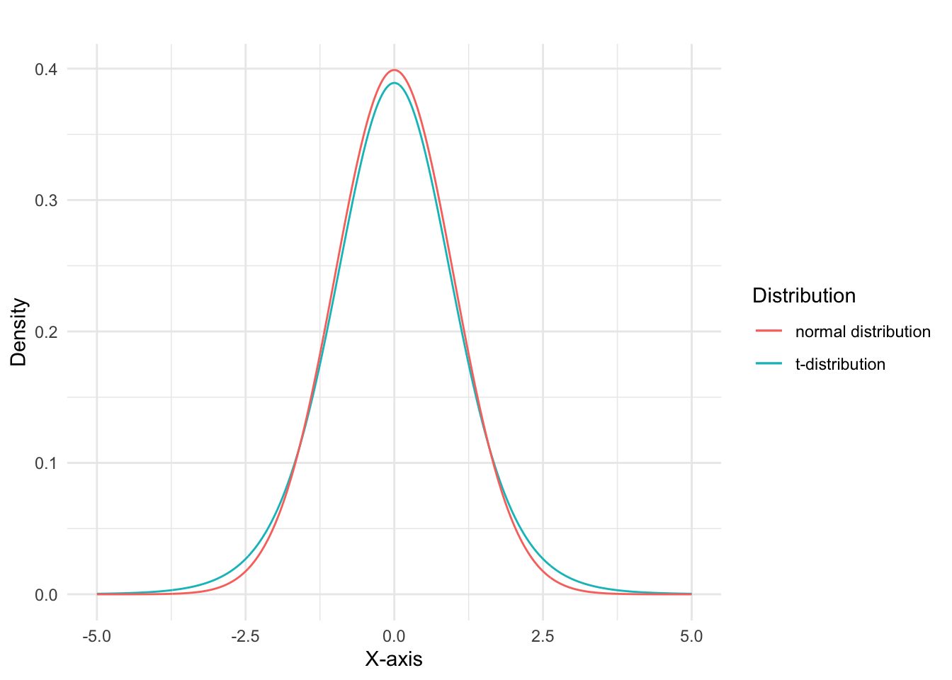
The t-distribution, also known as Student’s t-distribution, is a probability distribution that arises when estimating the mean of a normally distributed population with an unknown variance using a small sample. It is a continuous, symmetric distribution, similar to the standard normal distribution, but with thicker tails.
The t-distribution plays a crucial role in hypothesis testing, particularly in t-tests, which are used to compare sample means. When the population variance is unknown, which is often the case in real-world situations, the t-distribution is used to estimate the sampling distribution of the sample mean. The shape of the t-distribution is determined by a parameter called the degrees of freedom (df), which is related to the sample size. As the degrees of freedom increase, the t-distribution approaches the standard normal distribution.
Key features of the t-distribution:
Symmetry: Like the standard normal distribution, the t-distribution is symmetric around its mean, which is zero.
Thicker tails: The t-distribution has thicker tails compared to the standard normal distribution, implying a higher likelihood of observing extreme values or outliers. This feature is especially prominent with small sample sizes or low degrees of freedom.
Degrees of freedom: The t-distribution has a single parameter called degrees of freedom, which determines its shape. The degrees of freedom are typically defined as the sample size minus one (n-1) for a One-sample t-test or the sum of the sample sizes minus the number of groups for an independent samples t-test.
Convergence to the standard normal distribution: As the degrees of freedom (or sample size) increase, the t-distribution converges to the standard normal distribution. With large sample sizes, the difference between the two distributions becomes negligible, and the t-distribution can be approximated by the standard normal distribution.
The t-distribution is widely used in statistical analyses when the sample size is small and the population variance is unknown. Understanding the t-distribution is essential for conducting t-tests and interpreting their results accurately.
Code
# Load necessary librarieslibrary(ggplot2)# Set degrees of freedomdf <-10# Create a sequence of x valuesx <-seq(-5, 5, length.out =1000)# Calculate the density values for the t-distributiont_density <-dt(x, df)# Calculate the density values for the standard normal distributionnormal_density <-dnorm(x)# Create a data frame with the density valuesdata <-data.frame(x = x, t_density = t_density, normal_density = normal_density)# Plot the t-distribution and standard normal distributionggplot(data, aes(x)) +geom_line(aes(y = t_density, color ="t-distribution")) +geom_line(aes(y = normal_density, color ="normal distribution")) +labs(title ="",x ="X-axis",y ="Density",color ="Distribution") +theme_minimal()
Figure 1: Comparison of t-distribution and normal distribution
3 One-sample t-test
3.1 When to use it?
The One-sample t-test should be used when you have a single sample of data and you want to compare the mean of that sample to a known or hypothesized population mean.
3.2 Assumptions
The One-sample t-test makes several assumptions about the data:
Independence: The observations in the sample are independent of one another.
Normality: The population from which the sample is drawn is normally distributed.
Equal variances: The population variances of the two groups are equal.
Random sampling: The sample is drawn randomly and independently from the population.
Sample size: The sample size is large enough (usually greater than 30) for the Central Limit Theorem to be applied.
It is important to check these assumptions before running the One-sample t-test to ensure the validity of the test results. In case the sample size is small or the data distribution is not normal, a non-parametric test such as the Wilcoxon signed-rank test should be used instead.
3.3 Equation
Below are the two ways we can write the equation for the One-sample t-test.
\[
t = \frac{\bar{x} - \mu}{\frac{s}{\sqrt{n}}}
\tag{5}\]
where:
\(\bar{x}\) is the sample mean
\(\mu\) is the population mean
\(s\) is the sample standard deviation
\(n\) is the sample size
It also can be written as:
\[
t = \frac{\bar{x} - \mu}{s_x/\sqrt{n}}
\tag{6}\]
where:
\(\bar{x}\) is the sample mean
\(\mu\) is the population mean
\(s_x\) is the sample standard deviation
\(n\) is the sample size
3.4 Example
The kinesiologist wants to know if the mean muscle strength of the sample is significantly different from the population mean muscle strength of older adults (which is hypothesized to be 40 kg). The kinesiologist would run a One-sample t-test to compare the mean muscle strength of the sample (after completing the exercise program) to the hypothesized population mean of 40 kg. If the t-value is significant, the kinesiologist can conclude that the exercise program does improve muscle strength in older adults.
3.4.1 Research question
Do older adults improve muscle strength following a 8-week exercise program?
3.4.2 Hypotheses statements
To compare the mean of the After variable to a known value (in this case, 40), you can use the One-sample t-test. The hypotheses for the One-sample t-test comparing the mean After scores to the value of 40 can be stated as follows:
There is no significant difference between the mean After scores and the value 40. In other words, the population mean of the After scores is equal to 40.
There is a significant difference between the mean After scores and the value 40. In other words, the population mean of the After scores is not equal to 40.
3.4.3 Analyzing with jamovi
To run the One-sample t-test in jamovi, follow these steps:
Click the “hamburger” menu button (three horizontal lines) in the top-left corner of the jamovi window.
Click “Open” and then “This PC”
Locate and select “dynamometer.csv” and click “Open.”
Once the dataset is loaded, you’ll see the columns: Participant_ID, Age, Before, and After.
To run the One-sample t-test:
Click on the “Analyses” tab at the top of the jamovi window.
Click on the “T-Tests” dropdown menu, and then select “One-sample t-test.”
In the One-sample t-test window:
Drag the `After` variable from the left pane to the “Variable” box on the right pane.
In the “Test value” box, enter “40” (without quotes) as the hypothesized population mean.
You can select additional options such as “Mean difference” and “Effect size” under the “Statistics” dropdown if desired.
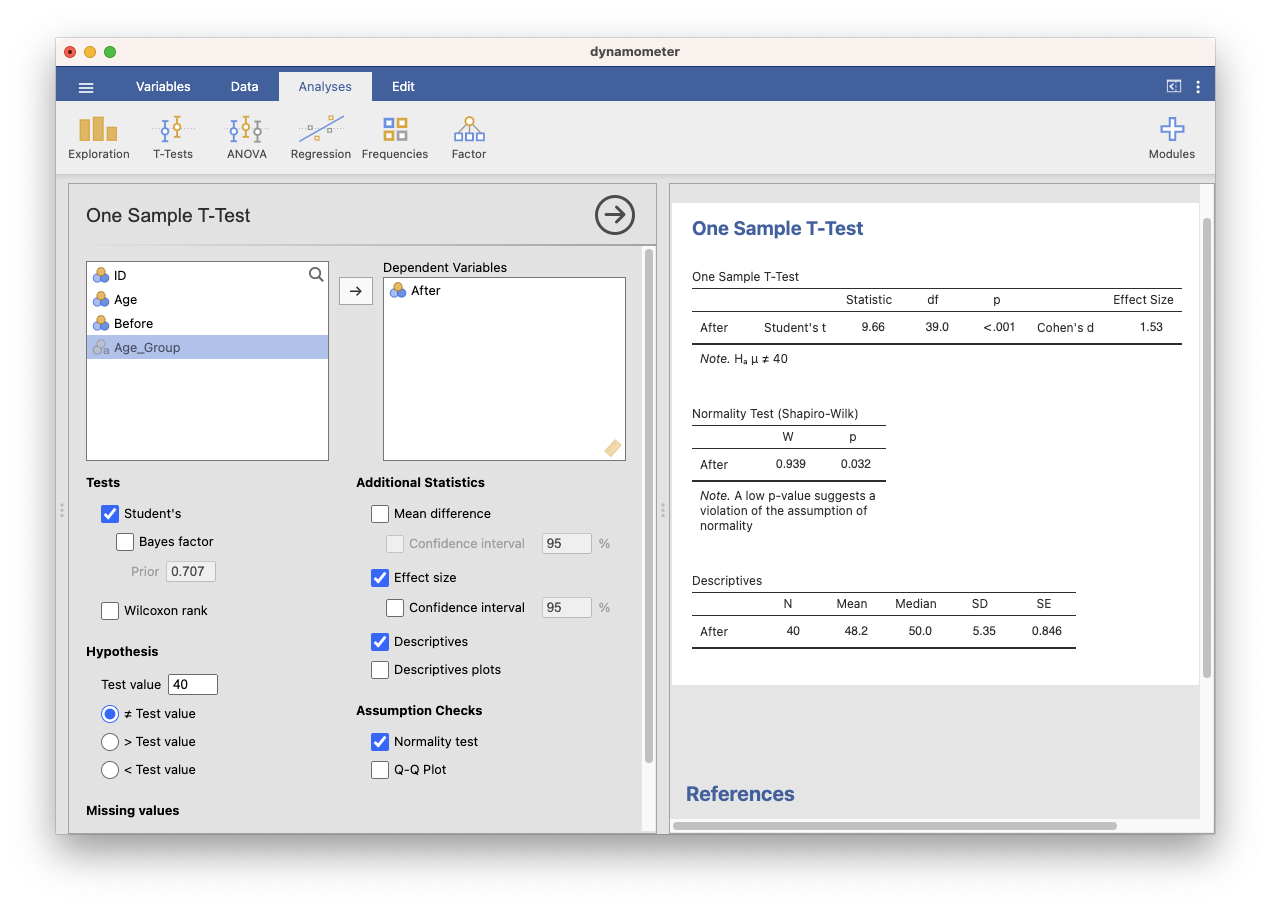
The One-sample t-test results will be displayed in the main window, including the t-value, degrees of freedom, p-value, and confidence interval. You can interpret the results to determine if the exercise program had a significant impact on muscle strength compared to the hypothesized population mean of 40 kg.
Remember to save your analysis for future reference by clicking “File” > “Save As” in the top-left corner of the jamovi window.
Click image to enlarge
Figure 2: One-sample t-test in jamovi
3.4.4 Analyzing with SPSS
To conduct a One-sample t-test in SPSS with the dynamometer data, follow these steps:
Open SPSS and load the dynamometer data into SPSS.
Click on “Analyze” in the top menu, and select “Compare Means” -> “One-Sample T Test”.
In the “One-Sample T Test” dialog box, select the variable After as the “Test Variable” and enter the hypothesized population mean of 40 kg in the “Test Value” field.
Click on the “Options” button and select the confidence level and effect size you wish to calculate (e.g., 95% confidence interval, Cohen’s d effect size).
Click “OK” to run the analysis.
SPSS will output the results of the One-sample t-test in a table. The table will include the sample mean, standard deviation, and standard error of the mean for the test variable, as well as the t-value, degrees of freedom, and p-value for the test. It will also include the confidence interval and effect size you selected in the “Options” dialog box.
Open the syntax editor by clicking on “File” > “New” > “Syntax.”
Copy and paste the syntax code provided above into the syntax editor.
Select all the lines of the syntax code.
Click on the green “Run” button or right-click and choose “Run Selection” to execute the syntax code.
The results will be displayed in the output window, just like when using the menu.
This syntax code performs the One-sample t-test comparing the After scores with a mean value of 40 and reports the results with a 95% confidence interval.
3.4.5 Analyzing with R
To calculate a One-sample t-test with R, you can follow these steps:
Load the data into R as a dataframe.
Use the t.test() function to conduct the One-sample t-test.
Specify the variable to be tested and the value of the population mean to be tested against.
Optional: specify the desired level of significance (alpha) and type of test (one-tailed or two-tailed).
Save the results of the t-test for future reference and use.
Code
# Read in the datamy_data <-read.csv("dynamometer.csv")# Subset the data for the variable of interestafter_data <- my_data$After# Run One-sample t-testt.test(after_data, mu=40)
    One Sample t-test

data:  after_data
t = 9.6577, df = 39, p-value = 6.798e-12
alternative hypothesis: true mean is not equal to 40
95 percent confidence interval:
 46.46284 49.88716
sample estimates:
mean of x
   48.175
3.4.6 Interpreting the results
Here are some steps to interpret the results for a one-sample t-test:
Check the assumptions of normality and homogeneity of variance.
Look at the t-test output and identify the test statistic, degrees of freedom, p-value, and confidence interval.
Evaluate the p-value. If the p-value is less than the alpha level (usually 0.05), then there is sufficient evidence to reject the null hypothesis.
Look at the confidence interval. If the confidence interval includes the null hypothesis value, then we cannot reject the null hypothesis. If the confidence interval does not include the null hypothesis value, then we can reject the null hypothesis.
Interpret the results in the context of the research question. State whether there is statistically significant evidence to support the hypothesis that the population mean differs from the null hypothesis value, and what the direction and magnitude of the difference is.
3.4.7 Reporting Results in APA Style
When reporting results of the one-sample t-test in APA Style, the following information should be included:
A description of the test used, including the name of the test (i.e., one-sample t-test), the sample size, and the level of significance (alpha) used.
A statement of the null and alternative hypotheses.
The test statistic (t-value) with degrees of freedom (df) and p-value.
The effect size, such as Cohen’s d, can be included as well.
A conclusion about whether the null hypothesis is rejected or failed to be rejected.
A discussion of the practical significance of the results and any limitations of the study.
For the current analysis, I will suggest the following:
A One-sample t-test was conducted to examine whether the new exercise program significantly improved muscle strength in older adults compared to the hypothesized population mean of 40 kg. The sample mean muscle strength after completing the exercise program was M = 48.2, SD = 5.35. The results revealed a statistically significant increase in muscle strength, t(39) = 9.66, p < .001, Cohen’s d = 1.53. The assumption of normality was violated, as indicated by a significant Shapiro-Wilk test, p = .032. Thus, the results should be interpreted with caution. Alternatively, you can run the Wilcoxon rank test, which is the non-parametric equivalent to the one-sample test.
Note
The statement above includes all the essential information in APA style: the test performed, the research question, the sample mean and standard deviation, the test statistic (t-value), the degrees of freedom (df), the p-value, the effect size (Cohen’s d), and the result of the normality test (Shapiro-Wilk).
3.4.7.1 Other Examples
The results of the one-sample t test indicated that the mean (M = X, SD = Y) was significantly different from the hypothesized value (t(df) = t-value, p < .05).
In a One-sample t test, the mean of the sample was significantly different from the hypothesized mean (t(df) = t-value, p < .05). Specifically, the mean of the sample was X (SD = standard deviation) while the hypothesized mean was Y.
The results of the one-sample t test indicated that the mean of the sample (M = X, SD = Y) was significantly different from the hypothesized mean (μ = t) t(df) = t-value, p < .05.
A one-sample t-test was conducted to determine whether the mean muscle strength score after the intervention (M = 42.5, SD = 3.2) differed significantly from the population mean of 40. The sample consisted of 20 participants, and the level of significance was set at alpha = .05. Results indicated that the mean muscle strength score was significantly higher than the population mean, t(19) = 2.57, p = .018, d = 0.64. Therefore, the null hypothesis was rejected. The effect size was small to medium. These findings suggest that the intervention was effective in improving muscle strength. However, the study is limited by the small sample size and the lack of a control group.
4 Independent-samples t-test
4.1 When to use it?
The Independent-samples t-test should be run when comparing the means of two independent groups. For example, in the field of kinesiology, an Independent-samples t-test can be used to compare the muscle strength of a group of individuals who have completed a resistance training program to a group of individuals who have not completed a resistance training program. The independent variable would be whether or not the individual completed the resistance training program and the dependent variable would be muscle strength. The t-test would be used to determine if there is a significant difference in muscle strength between the two groups, indicating that the resistance training program had an effect on muscle strength.
4.2 Assumptions
The assumptions of the Independent-samples t-test include:
Normality: The data should be approximately normally distributed within each group.
Independence: The observations in each group should be independent of one another.
Equal variances: The variances of the two groups should be roughly equal.
Random Sampling: The sample of each group should be random and representative of the population.
Equal sample size: The sample size in each group should be equal or similar.
It is important to note that not all these assumptions need to be perfectly met for the test to be valid, but the deviations from these assumptions should be small. If the data do not meet these assumptions, the non-parametric version of the Independent-samples t-test, such as the Mann-Whitney U test, can be used instead.
4.3 Effect size
Cohen’s d (cohen1988?) is a widely accepted measure of effect size for independent-samples t-tests. It is calculated by dividing the difference between the two group means by the pooled standard deviation of the two groups. The resulting value represents the number of standard deviations that separate the means of the two groups. The formula for Cohen’s d is:
\(n_1\) and \(n_2\) are the sample sizes of the two groups.
\(s_1\) and \(s_2\) are the sample standard deviations of the two groups.
For equal variance not assumed (Welch’s t-test):
\[
t = \frac{\bar{X}_1 - \bar{X}_2}{\sqrt{\frac{s_1^2}{n_1} + \frac{s_2^2}{n_2}}}
\]
\(t\) is the t-statistic.
\(\bar{X}_1\) and \(\bar{X}_2\) are the sample means of the two groups.
\(n_1\) and \(n_2\) are the sample sizes of the two groups.
\(s_1\) and \(s_2\) are the sample standard deviations of the two groups.
4.5 Example
In this example, the researcher wanted to investigate mean differences between the age groups.
4.5.1 Research question
Is there a significant difference in the mean After scores between the two age groups, 18-39 and 40-60, in terms of dynamometer performance?
4.5.2 Hypothesis statements
The hypotheses for this study, which aims to investigate the difference in the mean ‘After’ scores between the two age groups (18-39 and 40-60) in terms of dynamometer. performance, can be stated as follows:
There is no significant difference in the mean After scores between the two age groups (18-39 and 40-60) in terms of dynamometer performance. In other words, the mean After scores for the 18-39 age group are equal to the mean ‘After’ scores for the 40-60 age group.
There is a significant difference in the mean After scores between the two age groups (18-39 and 40-60) in terms of dynamometer performance. In other words, the mean After scores for the 18-39 age group are not equal to the mean. After scores for the 40-60 age group.
4.5.3 Analyzing with jamovi
Import the data:
Open Jamovi.
Click on the “Open” button in the top-left corner, navigate to the folder where your CSV file is located, and open the “dynamometer.csv” file. The data should now be displayed in the data view.
Perform the independent samples t-test:
Click on the “Analyses” tab in the top-left corner.
In the analyses menu, go to “T-Tests” and then click on “Independent Samples T-Test.” A new panel for the independent samples t-test will appear on the right side of the screen.
In the panel, drag and drop the After variable into the “Dependent Variable” box.
Drag and drop the Age_Group variable into the “Grouping Variable” box.
Set additional options (optional):
Check the desired options
In the example below, I chose Effect Size, Welch's, and Homogeneity test
View the results:
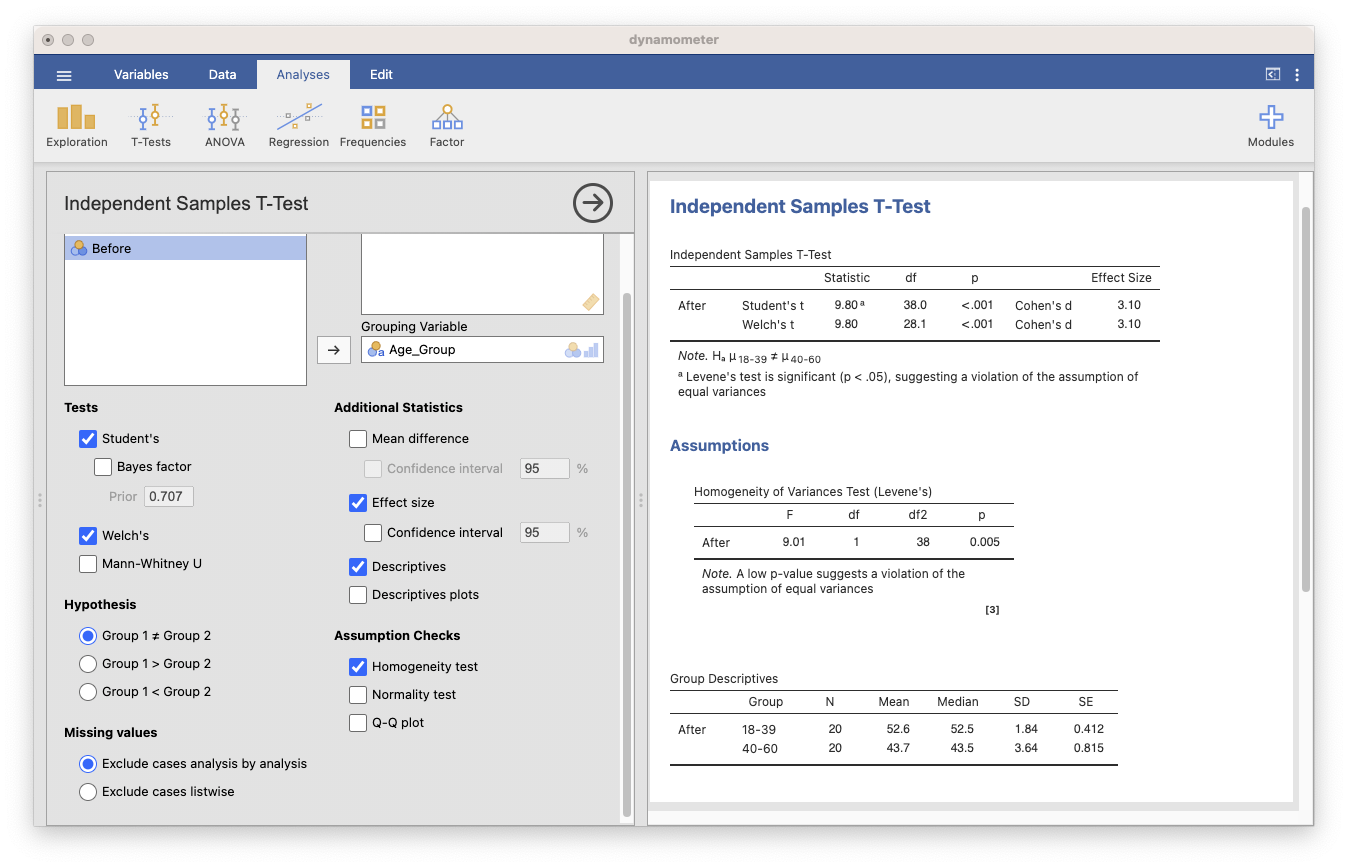
The results of the independent samples t-test will be displayed in the output pane on the right side of the screen. You’ll see the t-statistic, degrees of freedom, p-value, and confidence interval for the t-test. If you’ve selected the effect size option, Cohen’s d will also be displayed.
Figure 3: Independent-Samples t-test in jamovi
4.5.4 Analyzing with SPSS
To perform an independent samples t-test in SPSS, follow these steps:
Import the data:
Open SPSS.
Go to “File” > “Open” > “Data,” navigate to the folder where your CSV file is located, and open the “dynamometer.csv” file. The data should now be displayed in the data view.
If necessary, define the variable properties (e.g., labels, measurement level) in the “Variable View” tab at the bottom of the data window.
Perform the independent samples t-test using the menu:
Click on “Analyze” > “Compare Means” > “Independent-Samples T Test.”
In the “Independent-Samples T Test” dialog box, move the “Before” variable to the “Test Variable(s)” list.
Move the “Age_Group” variable to the “Grouping Variable” box.
Click on the “Define Groups” button and enter the group identifiers (e.g., “18-39” and “40-60”). Click “Continue.”
Click “OK” to run the independent samples t-test.
View the results:
The results of the independent-samples t-test will be displayed in the output window. You’ll see the t-statistic, degrees of freedom, p-value, and confidence interval for the t-test, as well as the results of Levene's test for the equality of variances.
Alternatively, you can use the syntax editor in SPSS to run the independent samples t-test. Here’s the syntax code:
* Load thedata.GET FILE='C:\path\to\your\data\dynamometer.sav'.* Conduct the Independent-samples t-test.T-TEST GROUPS=Age_Group(18-3940-60)/MISSING=ANALYSIS/VARIABLES=Before/CRITERIA=CI(.95).
To run the syntax code:
Open the syntax editor by clicking on “File” > “New” > “Syntax.”
Copy and paste the syntax code provided above into the syntax editor.
Select all the lines of the syntax code.
Click on the green “Run” button or right-click and choose “Run Selection” to execute the syntax code.
The results will be displayed in the output window, just like when using the menu.
This syntax code performs the independent samples t-test comparing the `After` scores between the two age groups (18-39 and 40-60) and reports the results with a 95% confidence interval.
4.5.5 Analyzing with R
Follow the instructions below to conduct an Independent-samples t-test to compare the After scores of the two age groups using the same data set:
Split the data set into two groups based on Age_Group column: “40-60” and “18-39”.
Calculate the means and standard deviations of After scores separately for each group.
Check if the assumption of equal variances is met by performing a Levene's test.
If the Levene's test is significant, use the Welch Two Sample t-test instead.
Conduct an Independent-samples t-test to compare the means of `After` scores between the two age groups.
Interpret the results, including the effect size using Cohen's d.
Here’s the R code to conduct the Independent-samples t-test:
Levene's Test for Homogeneity of Variance (center = median)
      Df F value Pr(>F)
group  1  8.8822  0.005 **
      38
---
Signif. codes:  0 '***' 0.001 '**' 0.01 '*' 0.05 '.' 0.1 ' ' 1
Levene's test is significant, suggesting unequal variances between the groups.

    Welch Two Sample t-test

data:  After by Age_Group
t = 9.8029, df = 28.128, p-value = 1.422e-10
alternative hypothesis: true difference in means between group 18-39 and group 40-60 is not equal to 0
95 percent confidence interval:
  7.080206 10.819794
sample estimates:
mean in group 18-39 mean in group 40-60
              52.65               43.70
To calculate the effect size for the Independent-samples t-test. Below, is the R code and calculation.
Code
# Calculate the means and standard deviations for each groupgroup_stats <- my_data %>%group_by(Age_Group) %>%summarise(Mean =mean(After), SD =sd(After), n =n())# Calculate the pooled standard deviationSD_pooled <-sqrt(((group_stats$n[1] -1) * group_stats$SD[1]^2+ (group_stats$n[2] -1) * group_stats$SD[2]^2) / (group_stats$n[1] + group_stats$n[2] -2))# Calculate Cohen's dcohens_d <- (group_stats$Mean[1] - group_stats$Mean[2]) / SD_pooled# Print Cohen's dcat("Cohen's d:", cohens_d, "\n")
Cohen's d: 3.099963
4.5.6 Interpreting the Results
When interpreting the results of an independent samples t-test, the following steps can be followed:
Check for the assumptions of normality and equal variances in each group. If these assumptions are not met, alternative tests or data transformations may need to be considered.
Examine the descriptive statistics and compare the means and standard deviations of each group.
Interpret the results of the Levene’s test to determine if there is a significant difference in variances between the two groups. A significant result suggests that the assumption of equal variances has been violated.
Interpret the results of the t-test. Look at the t-value, degrees of freedom, and p-value. The t-value indicates the magnitude of the difference between the means, the degrees of freedom indicate the sample size, and the p-value indicates the likelihood of obtaining the observed difference if there is truly no difference between the groups.
If the p-value is less than the chosen level of significance (usually 0.05), conclude that there is a significant difference between the means of the two groups. If the p-value is greater than the chosen level of significance, conclude that there is not enough evidence to support the claim of a difference between the means.
Consider the effect size, which provides an indication of the magnitude of the difference between the means. Common effect size measures include Cohen’s d and Hedges’ g. A larger effect size indicates a stronger difference between the groups.
Interpret the results in the context of the research question and any relevant literature.
4.5.7 Reporting Results in APA Style
When reporting the results of an independent-samples t test in APA style, the following information should be included:
The test statistic, degrees of freedom, and p-value. These values are typically reported in parentheses, such as (t(df) = t-value, p = p-value).
A description of the variables being compared, including the sample sizes and means for each group.
A statement of the null hypothesis and alternative hypothesis.
A brief interpretation of the results, including whether the null hypothesis was rejected or not.
A measure of effect size, such as Cohen’s d, may also be reported.
It is also a good idea to provide a brief interpretation of the results, explaining what they mean in the context of your research question or hypothesis.
For the current analysis, I suggest the following:
Based on an independent-samples t-test, there was a significant difference in “After” scores between the 18-39 (M = 52.6, SD = 1.84) and 40-60 (M = 43.7, SD = 43.5) age groups, t(28.1) = 9.80, p < .001, Cohen’s d = 3.10. Welch’s correction was used due to unequal variances.
4.5.8 Other Examples
An independent samples t-test was conducted to compare the mean scores of two groups on a measure of stress. The sample consisted of 20 participants in Group A and 25 participants in Group B. The mean score for Group A was M = 3.5, SD = 1.2, and the mean score for Group B was M = 2.8, SD = 0.9. The t-value was t(43) = 2.3, p = .03, indicating that there was a significant difference between the mean scores of the two groups, with Group A scoring higher than Group B. The effect size for the difference between the two groups was d = .7, indicating a moderate effect. These results suggest that participants in Group A experienced significantly higher levels of stress than those in Group B.
The purpose of this study was to examine the effect of a new teaching method on student achievement. A sample of 50 students was randomly assigned to either the experimental group, which received the new teaching method, or the control group, which received the traditional teaching method. Student achievement was measured using a standardized test. The results of the independent samples t-test showed that there was a statistically significant difference between the experimental and control groups, t(48) = 2.57, p = .01. The experimental group had a higher mean score on the achievement test than the control group. These findings suggest that the new teaching method was effective in improving student achievement. However, it is important to note that the small sample size and lack of generalizability to other populations are limitations of this study.
5 Paired-samples t-test
5.1 When to use it?
The Paired-samples t-test should be run when you have two sets of related (or paired) data that you want to compare. For example, if you want to compare the effectiveness of two different treatments on a group of patients, you would use a Paired-samples t-test. This test is also commonly used in pre- and post-test designs, where you want to compare scores before and after an intervention or treatment. Additionally, if you want to compare the mean differences between two groups or conditions, but you want to control for individual differences, you can use a Paired-samples t-test.
5.2 Assumptions
The assumptions of the Paired-samples t-test include:
Independence: The observations within each pair are independent of one another.
Normality: The differences between the pairs of observations are approximately normally distributed.
Equal variances: The variances of the differences between the pairs of observations are equal.
Paired data: The observations are paired, meaning that each individual is measured twice, once before and once after some intervention, or in two different conditions.
Random Sampling: The sample being used is selected randomly from the population.
It’s important to note that violations of these assumptions may lead to inaccurate results, so it’s necessary to check them before applying the test. Checking for normality can be done using a normal probability plot, and checking for equal variances can be done using Levene’s test. The paired sample t-test is sensitive to the violation of normality and equal variances assumptions, thus if the assumptions are not met, there are other options that can be used, such as the Wilcoxon signed-rank test which is a non-parametric version of the Paired-samples t-test.
5.3 Equation
\[
t = \frac{\bar{d}}{s_d/\sqrt{n}}
\]
where, \(\bar{d}\) is the mean difference, \(s_d\) is the standard deviation of the differences, \(n\) is the sample size, \(t\) and is the t-statistic.
5.4 Example
A researcher wanted to investigate whether an intervention (such as an exercise program) has a significant effect on muscle strength. Participants were recruited based on specific inclusion criteria (e.g., age range, health status, etc.), and muscle strength measurements (in kg) were taken for each participant both before and after the intervention. The null hypothesis would be that there is no significant difference between the “Before” and “After” measurements, while the alternative hypothesis would be that there is a significant difference. The Paired-samples t test would be an appropriate statistical analysis to test this hypothesis.
5.4.1 Research Question
Is there a significant difference between muscle strength before and after a training program among participants of different age groups?
5.4.2 Hypotheses Statements
There is no significant difference between the mean of the differences in the paired observations. In other words, the mean difference between the ‘Before’ and ‘After’ scores is equal to zero.
There is a significant difference between the mean of the differences in the paired observations. In other words, the mean difference between the ‘Before’ and ‘After’ scores is not equal to zero.
Click the “hamburger” menu button (three horizontal lines) in the top-left corner of the jamovi window.
Click “Open” and then “This PC”
Locate and select “dynamometer.csv” and click “Open.”
Once the dataset is loaded, you’ll see the columns: ID, Age, Before, and After.
Click the “T-tests” button on the top of the screen and select “Paired Samples t-test” from the dropdown menu.
A new window will appear, displaying the Paired-samples t-test options. Move the Before and After variables under Paired Variables.
Select the options option shown in the screenshot below.
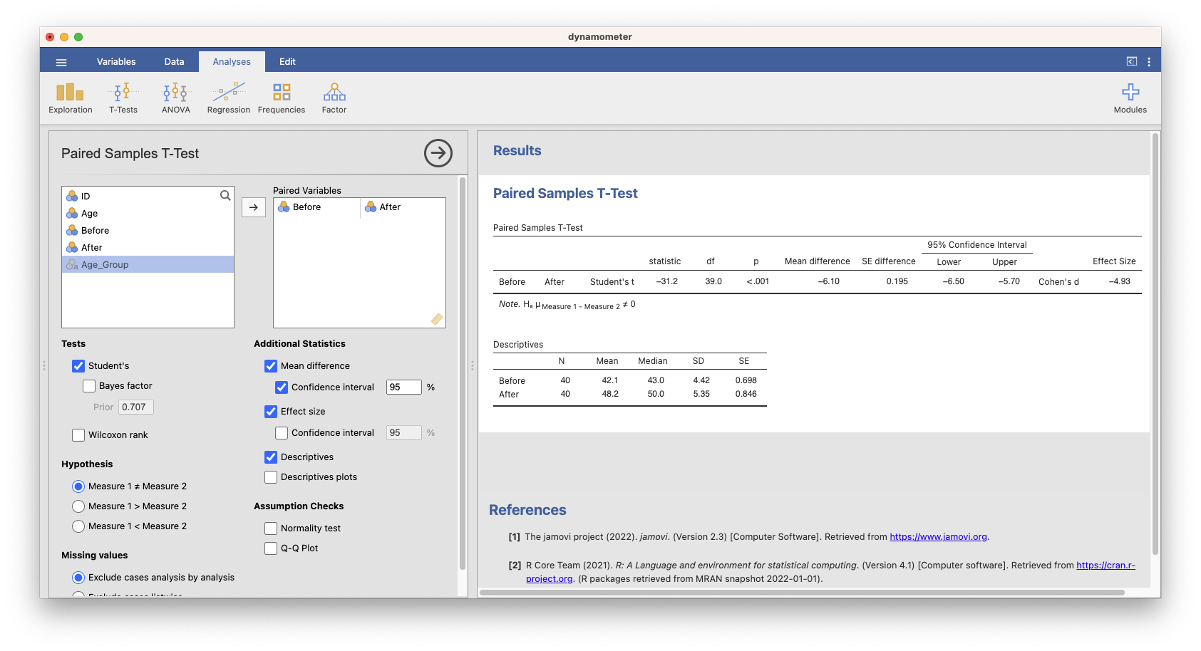
The results will appear in the “Results” tab on the right side of the screen, including means, standard deviations, the t-value, degrees of freedom, and the p-value.
Conducting the Paired-samples t-test in jamovi
5.4.4 Analyzing with SPSS
here are the steps to run the Paired-samples t-test in SPSS:
Open SPSS and go to File > Open > Data.
Locate the dynamometer.csv file and click Open.
Select the option “Read variable names from the first row of data” and click OK.
Go to Analyze > Compare Means > Paired-samples T Test.
In the “Paired Variables” dialog box, select “Before” and “After” and move them to the “Paired Variables” list using the arrow button.
Click the “Options” button and select “Descriptive statistics” and “Paired samples test” checkboxes.
Click the “Continue” button and then click the “OK” button to run the analysis.
Here is the syntax for the Paired-samples t-test in SPSS:
Note that the GET command should be modified to specify the correct file path for the “dynamometer.csv” data set. Also, the COMPUTE command creates a new variable called “Before_After” that represents the difference between the “After” and “Before” variables. The T-TEST command then conducts the Paired-samples t-test using the “Before_After” variable, with the OPTIONS subcommand specifying the desired confidence level and requesting descriptive statistics and effect size measures.
To run the syntax in SPSS, you can follow these steps:
Open SPSS and go to “File” -> “Open” -> “Data”.
In the “Open Data” window, locate and select the “dynamometer.sav” file.
Click “Open” and the data set will be loaded into SPSS.
Go to “File” -> “New” -> “Syntax”.
In the syntax editor, copy and paste the syntax provided earlier.
Click “Run” to execute the syntax.
The output will be displayed in the output viewer.
5.4.5 Analyzing with R
Here are the steps to run a Paired-samples t-test in RStudio using the dynamometer.csv data set.
Running the text
Code
# Load the datamy_data <-read.csv("dynamometer.csv")# Calculate the differences between 'Before' and 'After' scoresmy_data$Difference <- my_data$After - my_data$Before# Run the paired samples t-testt_test_result <-t.test(my_data$Before, my_data$After, paired =TRUE)# Print the t-test resultprint(t_test_result)
    Paired t-test

data:  my_data$Before and my_data$After
t = -31.208, df = 39, p-value < 2.2e-16
alternative hypothesis: true mean difference is not equal to 0
95 percent confidence interval:
 -6.495358 -5.704642
sample estimates:
mean difference
           -6.1
To interpret the results of a paired samples t-test and the effect size (Cohen’s d), follow these steps:
Check the t-test’s p-value: The p-value indicates the probability of observing a test statistic as extreme as the one obtained if the null hypothesis were true. In this case, the null hypothesis states that there is no significant difference between the “Before” and “After” scores.
If the p-value is less than the significance level (usually set at 0.05), you can reject the null hypothesis and conclude that there is a significant difference between the “Before” and “After” scores.
If the p-value is greater than the significance level, you cannot reject the null hypothesis and there is insufficient evidence to conclude that there is a significant difference between the “Before” and “After” scores.
Evaluate Cohen’s d: Cohen’s d is a measure of the effect size, which indicates the standardized magnitude of the difference between the “Before” and “After” scores. The larger the absolute value of Cohen’s d, the larger the effect size.
Small effect: |d| = 0.2
Medium effect: |d| = 0.5
Large effect: |d| = 0.8
These are general guidelines for interpreting Cohen’s d. Depending on the context of your study, these thresholds may vary.
5.4.7 Reporting Results
When reporting the results of a Paired-samples t-test, it is important to include the following information:
The test statistic (e.g. t-value) and the associated p-value. The t-value tells us how many standard errors the mean difference is from zero, and the p-value tells us the probability of observing a t-value as extreme as the one we calculated under the assumption that the null hypothesis is true.
The sample size (e.g. the number of pairs of observations).
The mean difference and the standard deviation of the differences.
The effect size, such as Cohen’s d, which is a measure of the magnitude of the difference between the means.
For the current analysis, I suggest the following:
A Paired-samples t-test was conducted to compare the scores before and after the intervention. There was a significant difference in the scores for before (M = 42.1, SD = 4.42) and after (M = 48.2, SD = 5.35) conditions; t(39) = -31.208, p < .001, 95% CI [-6.495, -5.705], Cohen’s d = 4.93. The results indicate that there is a significant difference between the “Before” and “After” scores, with the “After” scores being higher on average. The effect size (Cohen’s d) is large, suggesting that the intervention had a substantial impact on the scores.
5.4.8 Other Examples
A Paired-samples t-test was conducted to compare the pre-test and post-test scores of a group of students. The sample size was 20 pairs of observations. The mean difference between the pre-test and post-test scores was 5.3 (SD = 2.5). The t-value was 3.87, with a p-value of 0.001. The effect size (Cohen’s d) was 0.67, which indicates a moderate effect size.
The results of the Paired-samples t-test revealed that there was a statistically significant difference between the pre-test and post-test scores of the students, t(19) = 3.87, p = 0.001. The mean difference was 5.3 (95% CI [3.4, 7.2]), and the effect size (d = 0.67) suggests moderate effect size.