Understand the basic concepts of one-way ANOVA, including independent and dependent variables, group comparisons, and null and alternative hypotheses.
Learn how to perform a one-way ANOVA using R, SPSS, and jamovi.
Understand how to interpret the output from a one-way ANOVA, including the F statistic, p-value, and effect size.
Learn how to conduct post-hoc analyses, including pairwise comparisons, to examine specific group differences.
Understand the assumptions underlying one-way ANOVA and how to check for their violation.
Learn how to report the results of a one-way ANOVA in APA format.
1 Sample data
This dataset consists of 45 participants divided into three exercise programs (A, B, and C). Each participant’s flexibility was measured at three time points (Time1, Time2, and Time3). Additionally, the dataset includes information about each participant’s gender (Male or Female).
pacman::p_load("tidyverse", "dplyr", "psych", "knitr", "kableExtra")# Read the datasetdata <-read.csv("flexibility.csv", header =TRUE)# Convert Group and Gender to factorsdata$Group <-as.factor(data$Group)data$Gender <-as.factor(data$Gender)# Compute the descriptives tabledescriptives <- data %>%select(Group, Gender, Flex_Time1, Flex_Time2, Flex_Time3) %>%group_by(Group, Gender) %>% psych::describe() %>%select(-n, -se)# Print the descriptives table in a nice formatkable(descriptives)
vars
mean
sd
median
trimmed
mad
min
max
range
skew
kurtosis
Group*
1
2.000000
0.8257228
2
2.000000
1.4826
1
3
2
0.0000000
-1.5659259
Gender*
2
1.555556
0.5025189
2
1.567568
0.0000
1
2
1
-0.2161948
-1.9961481
Flex_Time1
3
27.511111
5.1769692
27
27.216216
5.9304
20
39
19
0.4549922
-0.8968789
Flex_Time2
4
30.022222
5.2418287
29
29.756757
5.9304
22
41
19
0.4228177
-0.9456558
Flex_Time3
5
33.022222
5.2418287
32
32.756757
5.9304
25
44
19
0.4228177
-0.9456558
2 Intro to one-way ANOVA
One-way Analysis of Variance (ANOVA) is a statistical technique used to compare the means of three or more groups. It is an extension of the t-test, which can only compare the means of two groups. The main purpose of one-way ANOVA is to determine if there are any significant differences among the group means.
One-way ANOVA tests the null hypothesis (H0) that all group means are equal against the alternative hypothesis (H1) that at least one group mean is different. It does not tell us which specific group means are different, but rather whether there is sufficient evidence to conclude that there is a significant difference among the groups. If the null hypothesis is rejected, post-hoc tests can be conducted to identify the specific group differences.
3 Equation
In a one-way Analysis of Variance (ANOVA), the main goal is to determine whether there are statistically significant differences between the means of multiple groups. To do this, we examine the variability in the data, which is partitioned into two components: Sum of Squares Between groups (SSB) and Sum of Squares Within groups (SSW).
Sum of Squares Between groups (SSB): SSB measures the variability between the group means. It quantifies the differences in the means of the different groups compared to the grand mean, which is the overall mean of all data points across all groups. A larger SSB value indicates a greater difference between the group means, suggesting that the factor being studied may have a significant impact on the outcome.
Sum of Squares Within groups (SSW): SSW, on the other hand, measures the variability within each group. It represents the dispersion or spread of individual data points around their respective group means. A larger SSW value indicates more variability within the groups, which may be due to random errors or other factors not accounted for in the study.
The key differences between SSB and SSW are:
SSB is concerned with the variability between group means, while SSW focuses on the variability within each group.
SSB helps identify the effect of the factor being studied (e.g., a treatment or intervention) on the outcome, whereas SSW accounts for random errors and other unexplained factors affecting the data.
In a one-way ANOVA, these two components of variability are used to calculate the F-ratio, which is the test statistic for determining whether the differences between the group means are statistically significant. The F-ratio is calculated as the ratio of the Mean Square Between groups (MSB = SSB / degrees of freedom between groups) to the Mean Square Within groups (MSW = SSW / degrees of freedom within groups). A larger F-ratio indicates that the between-group variability is greater than the within-group variability, suggesting that the differences between the group means are statistically significant.
3.1 Calculate the sum of squares:
Sum of squares is calculated using the following components:
Sum of squares between groups (SSB): It measures the variability among group means.
\[
SSB = Σk(Ŷi. - Ŷ..)² / ni
\]
where k is the number of groups, Ŷi. is the mean of group i, Ŷ.. is the grand mean, and ni is the number of observations in group i.
Sum of squares within groups (SSW): It measures the variability within each group.
\[
SSW = ΣΣ(Yij - Ŷi.)²
\]
where Yij is the observation j in group i, and Ŷi. is the mean of group i.
Total sum of squares (SST): It measures the total variability in the data.
\[
SST = ΣΣ(Yij - Ŷ..)²
\]
3.2 Calculate the F-ratio
The F-ratio is calculated using the mean squares, which are obtained by dividing the sum of squares by their respective degrees of freedom.
Mean squares between groups (MSB):
\[
MSB = SSB / (k - 1)
\]
where k is the number of groups.
Mean squares within groups (MSW):
\[
MSW = SSW / (N - k)
\]
where N is the total number of observations.
F-ratio:
\[
F = MSB / MSW
\]
The F-ratio follows an F-distribution with (k - 1) and (N - k) degrees of freedom. The F-ratio is then compared to the critical value from the F-distribution table at a given significance level (usually α = 0.05) to determine if the null hypothesis can be rejected.
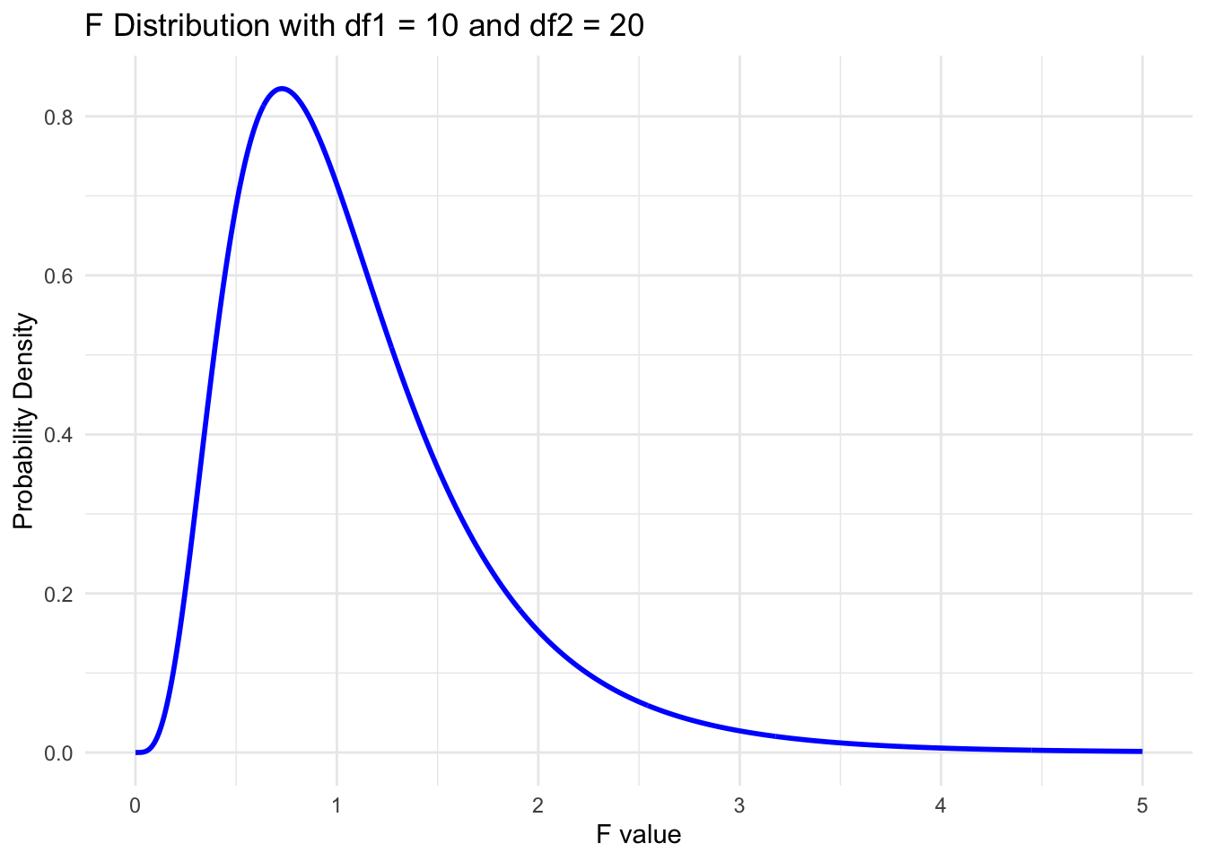
4 F Distribution
The F distribution, also known as the Fisher-Snedecor distribution, is a continuous probability distribution that is widely used in statistical hypothesis testing, particularly in the analysis of variance (ANOVA). It is named after Ronald A. Fisher and George W. Snedecor, two prominent statisticians who contributed significantly to its development.
4.1 Characteristics of the F Distribution
The F distribution has two important parameters: degrees of freedom for the numerator (df1) and degrees of freedom for the denominator (df2). These parameters define the shape of the distribution. Some key characteristics of the F distribution are:
It is always non-negative, as it represents the ratio of two chi-square distributions.
It is asymmetric and positively skewed, with a longer tail on the right side.
The peak of the distribution shifts to the right as the degrees of freedom increase.
As both degrees of freedom approach infinity, the F distribution converges to a normal distribution.
4.2 Applications of the F Distribution in ANOVA
The F distribution is central to the analysis of variance (ANOVA) and other statistical tests that involve comparing variances or assessing the effects of different factors on a response variable. In these applications, an F statistic is calculated as the ratio of two mean square values (MS), which are derived from sums of squares (SS) and degrees of freedom:
F = (MS_between groups) / (MS_within groups)
The numerator (MS_between groups) represents the variability between the groups, while the denominator (MS_within groups) represents the variability within the groups. If there is no significant difference between the groups, the F statistic should be close to 1. However, if the variability between the groups is much larger than the variability within the groups, the F statistic will be much greater than 1, indicating a significant effect of the factor being tested.
In hypothesis testing, the calculated F statistic is compared to a critical value from the F distribution with the appropriate degrees of freedom. If the F statistic exceeds the critical value, the null hypothesis is rejected, suggesting that there is a significant effect of the factor being tested.
In summary, the F distribution is a crucial tool in the analysis of variance and other statistical tests that involve comparing variances or assessing the effects of different factors on a response variable. Understanding its characteristics and applications can help you better interpret the results of your statistical analyses.
Code
# Load required packages quietlyif (!require("pacman")) install.packages("pacman", quiet =TRUE)suppressMessages(pacman::p_load("ggplot2", "ggthemes"))# Set the parameters for the F distributiondf1 <-10# degrees of freedom for the numeratordf2 <-20# degrees of freedom for the denominator# Create a function to calculate the probability density function (pdf) of the F distributionf_pdf <-function(x) {df(x, df1, df2)}# Define the range of x values to plotx_range <-seq(0, 5, length.out =1000)# Plot the F distribution using ggplot2suppressWarnings(ggplot(data.frame(x = x_range, y =f_pdf(x_range)), aes(x = x, y = y)) +geom_line(color ="blue", size =1) +ggtitle(paste("F Distribution with df1 =", df1, "and df2 =", df2)) +xlab("F value") +ylab("Probability Density") +theme_minimal())
5 Measure of effect size
There are a few different measures of effect size that can be used with a one-way ANOVA, depending on your research question and the specific context of your study. Some commonly used measures of effect size for one-way ANOVA include eta-squared (\(\eta^2\)), partial eta-squared (\(\eta_p^2\)), and omega-squared (\(\omega^2\)).
5.1 Eta-squared (\(\eta^2\))
\(\eta^2\) is the most commonly used measure of effect size for one-way ANOVA. It represents the proportion of variance in the dependent variable that is explained by the independent variable. It ranges from 0 to 1, with higher values indicating a stronger effect.
Equation
\[\eta^2 = \frac{SS_{between}}{SS_{total}}\]
Interpretation
(\(\eta^2\)): ranges from 0 to 1, with larger values indicating a stronger effect. A common rule of thumb is to consider values of 0.01, 0.06, and 0.14 to represent small, medium, and large effect sizes, respectively. For example, if you calculated an \(\eta^2\) value of 0.15 for your one-way ANOVA, you could interpret this as a large effect size.
Partial eta-squared (\(\eta_p^2\))
\(\eta_p^2\) is a variation of eta-squared that takes into account the degrees of freedom associated with the residual error term. It is sometimes preferred over eta-squared because it can be less biased in situations where the sample size is small or the assumptions of the ANOVA are violated.
Like eta-squared, partial eta-squared ranges from 0 to 1, with larger values indicating a stronger effect. However, partial eta-squared is adjusted for the degrees of freedom associated with the residual error term, so it can be less biased than eta-squared in certain situations. The same rule of thumb for interpreting eta-squared values can be applied to partial eta-squared.
5.2 Omega-squared (\(\omega^2\))
\(\omega^2\) is another measure of effect size that is similar to eta-squared, but it attempts to estimate the true population effect size rather than the effect size in the sample. It is typically used when the sample size is relatively small and/or the population effect size is unknown.
Omega-squared ranges from 0 to 1, with larger values indicating a stronger effect. However, because omega-squared attempts to estimate the true population effect size rather than the effect size in the sample, it may be more appropriate to use a slightly different rule of thumb for interpreting its values. One commonly used guideline is to consider values of 0.01, 0.06, and 0.14 to represent small, medium, and large effect sizes, respectively, but note that these thresholds are somewhat arbitrary and may vary depending on the specific context of your study.
In these equations, \(SS_{between}\) represents the sum of squares between groups, \(SS_{total}\) represents the total sum of squares, \(SS_{error}\) represents the sum of squares error (also known as the residual sum of squares), \(df_{between}\) represents the degrees of freedom between groups, and \(MS_{error}\) represents the mean square error (calculated as \(SS_{error} / df_{error}\)).
6 Post-hoc analysis
A one-way ANOVA is a powerful statistical method used to determine whether there are significant differences among the means of three or more independent groups. When the ANOVA test reveals a significant difference, it is necessary to perform post-hoc tests to identify the specific pairs of group means that significantly differ from one another. In this blog post, we will explore the role of post-hoc tests in a one-way ANOVA, the common post-hoc tests used, and the factors to consider when selecting the appropriate test.
A significant F-ratio in a one-way ANOVA indicates that there is a significant difference among the group means. However, it does not provide information about which specific group means are significantly different. This is where post-hoc tests come into play. These tests are designed to perform pairwise comparisons between the groups to determine which pairs of group means significantly differ while controlling the experiment-wise Type I error rate.
There are several post-hoc tests available, each with its advantages and limitations. Some of the most commonly used post-hoc tests include:
Tukey’s HSD (Honestly Significant Difference) Test: This test is widely used for pairwise comparisons when the assumption of equal variances is met. It controls the experiment-wise Type I error rate and is considered one of the most powerful tests when sample sizes are equal.
Bonferroni Test: This test adjusts the significance level (alpha) by dividing it by the number of pairwise comparisons. While it is more conservative than Tukey’s HSD test, it can be applied regardless of whether the sample sizes are equal or unequal.
Scheffé’s Test: This test is more conservative than Tukey’s HSD and the Bonferroni test but allows for any linear combination of means (not just pairwise comparisons). It is appropriate when conducting complex planned comparisons.
Games-Howell Test: This test is specifically designed for situations where the assumption of equal variances is not met (heteroscedasticity). It uses the Welch-Satterthwaite degrees of freedom to account for unequal variances and is a suitable choice when the assumption of equal variances is violated.
When selecting the appropriate post-hoc test, several factors need to be considered:
Assumption of Equal Variances: If the assumption of equal variances is met, Tukey’s HSD, Bonferroni, or Scheffé’s test may be appropriate. If this assumption is violated, the Games-Howell test is a suitable choice.
Sample Sizes: If sample sizes are equal, Tukey’s HSD is a powerful option. If sample sizes are unequal, the Bonferroni test or Games-Howell test (if the assumption of equal variances is violated) can be considered.
Conservativeness vs. Power: Different post-hoc tests offer varying levels of conservativeness and power. Tukey’s HSD is more powerful but less conservative, while the Bonferroni and Scheffé’s tests are more conservative but less powerful. Balancing the trade-off between Type I and Type II error rates is essential when selecting the appropriate post-hoc test.
7 Result interpretation
When you run a one-way ANOVA in R, you’ll typically get output that includes information on the degrees of freedom associated with the between-group factor (i.e., the “Group” variable in your case), the degrees of freedom associated with the residual error term, the sum of squares for the between-group factor, the sum of squares for the residual error term, the mean squares for the between-group factor and the residual error term, the F-statistic, and the p-value associated with the F-statistic.
To interpret the results of the one-way ANOVA, you’ll want to look at both the F-statistic and the associated p-value. The F-statistic indicates whether there are significant differences between the group means, while the p-value tells you whether those differences are statistically significant. If the p-value is less than your chosen alpha level (e.g., 0.05), then you can conclude that there is evidence of a significant difference between at least two of the group means.
In addition to looking at the statistical significance of the one-way ANOVA, you may also want to examine the effect size associated with the analysis. As I mentioned earlier, common effect size measures for a one-way ANOVA include eta-squared (\(\eta^2\)), partial eta-squared (\(\eta_p^2\)), and omega-squared (\(\omega^2\)). These effect size measures provide information on the magnitude of the differences between the group means. Generally, larger effect sizes indicate more meaningful differences between the groups.
In summary, when interpreting the results of a one-way ANOVA in R, you’ll want to look at both the statistical significance of the F-test and the associated p-value, as well as the effect size measures to determine the magnitude of the differences between the group means.
8 One-Way ANOVA Example
Using the sample dataset provided earlier, we will now perform a one-way ANOVA to determine if there is a significant difference in flexibility among the three exercise programs.
8.1 Research question
Is there a significant difference in flexibility among participants in the three different exercise programs (A, B, and C)?
For α = 0.05 and degrees of freedom (2, 12), the critical value from the F-distribution table is approximately 3.89.
Compare the F-ratio to the critical value:
Since the calculated F-ratio (0.925) is less than the critical value (3.89), we fail to reject the null hypothesis. This means that there is not enough evidence to conclude that there is a significant difference in flexibility among the three exercise programs.
In summary, one-way ANOVA is a powerful statistical technique for comparing the means of three or more groups. By understanding the underlying concepts and equations, kinesiology professionals can apply this method to their research and draw meaningful conclusions about the effects of various interventions on human movement and health.
8.4 Analyzing with jamovi
Here are the steps to analyze the provided dataset using jamovi:
Import the dataset:
First, open jamovi and click on the ‘open’ button in the top-left corner.
Browse your computer to find the CSV file containing the dataset, select it, and click ‘Open.’
The dataset should now be displayed in the jamovi data editor.
Conduct the one-way ANOVA:
Click on the ‘Analyses’ tab in the top-left corner of the jamovi window.
In the ‘Analyses’ panel on the left side, click on the ‘ANOVA’ section, and then select ‘One-Way ANOVA.’
In the ‘One-Way ANOVA’ options panel, drag and drop the ‘Flexibility’ variable into the ‘Dependent Variable’ box and the ‘Group’ variable into the ‘Fixed Factors’ box.
Select additional options (if desired):
Under the ‘Assumption Checks’ section, you can select ‘Homogeneity tests’ to check for the homogeneity of variances assumption (Levene’s test).
Under the ‘Post Hoc Tests’ section, you can select a post hoc test (e.g., Tukey, Bonferroni, or Scheffé) to perform pairwise comparisons between the groups if you find a significant overall effect.
Interpret the results:
After completing the steps above, jamovi will display the results of the one-way ANOVA in the right panel.
Look for the ‘ANOVA’ table, which includes the F-ratio, degrees of freedom, p-value, and other relevant information.
Compare the calculated p-value with your chosen significance level (usually α = 0.05). If the p-value is less than α, you can reject the null hypothesis and conclude that there is a significant difference in flexibility among the exercise programs.
Interpret post hoc tests (if applicable):
If you selected a post hoc test and found a significant overall effect, examine the post hoc test results to determine which specific group means are significantly different from each other.
By following these steps, you can analyze the provided dataset using one-way ANOVA in jamovi and draw meaningful conclusions about the differences in flexibility among the three exercise programs.
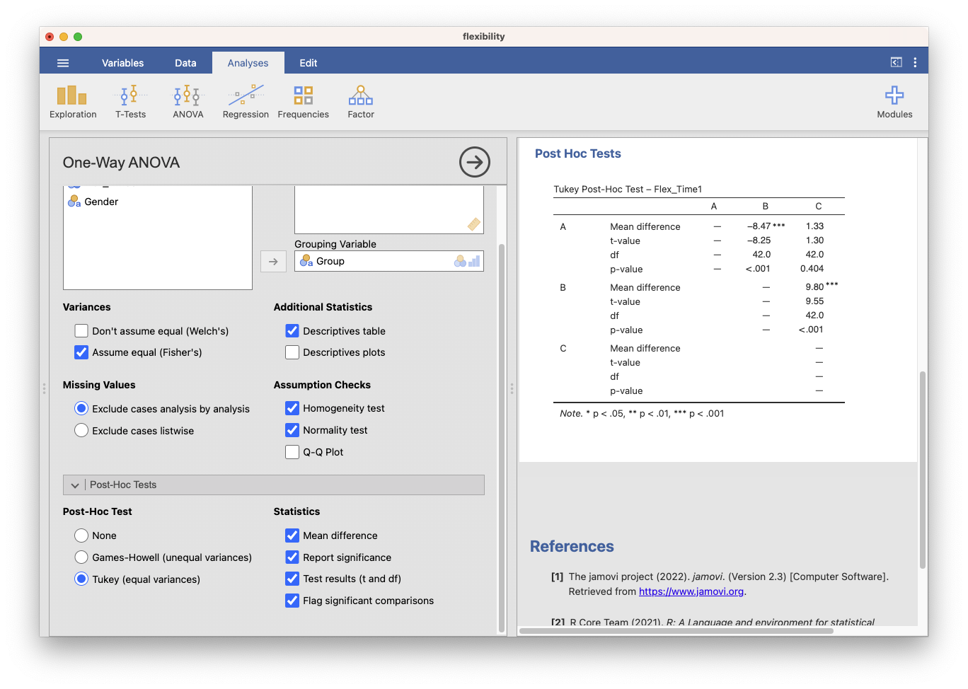
Figure 1: One-way ANOVA Omnibus set up and results
Figure 2: jamovi One-way ANOVA post-hoc set and results
8.5 Analyzing with SPSS
Here are the steps to perform a one-way ANOVA in SPSS.
Load your data into SPSS. Ensure that your data file is in the appropriate format (e.g., CSV or Excel). You can open your dataset by selecting File > Open > Data... and then browsing to your file.
Once your data is loaded, click on Analyze > Compare Means > One-Way ANOVA.
In the “One-Way ANOVA” dialog box, move the dependent variable (e.g., “Flex_Time1”) to the “Dependent List” box and the independent variable (e.g., “Group”) to the “Factor” box.
If you want to perform post hoc tests, click on the Post Hoc... button, select the desired post hoc test(s) (e.g., Tukey), and click Continue.
Click OK to run the one-way ANOVA. The results will be displayed in the output window.
Replace 'path/to/your/flexibility.csv' with the actual path to your dataset file. The first block of code loads the dataset into SPSS, and the second block of code performs the one-way ANOVA with post hoc Tukey test. The output will provide you with the necessary test statistics, such as the F-value and p-value, to help you determine whether there is a significant difference between the group means.
8.6 Analyzing with R
These steps will guide you through conducting a one-way ANOVA in RStudio. The output will provide you with the necessary test statistics, such as the F-value and p-value, to help you determine whether there is a significant difference between the group means.
Code
# Load required packagesif (!require("pacman")) install.packages("pacman", quiet =TRUE)suppressMessages(pacman::p_load("tidyverse", "ggplot2", "ggthemes", "broom"))# Load the datasetdata <-read.csv("flexibility.csv")# Ensure that the "Group" variable is a factordata$Group <-as.factor(data$Group)# Perform the one-way ANOVAanova_results <-aov(Flex_Time1 ~ Group, data = data)# Display the summary of the ANOVA resultssummary(anova_results)
            Df Sum Sq Mean Sq F value   Pr(>F)
Group        2  847.5   423.8   53.65 2.71e-12 ***
Residuals   42  331.7     7.9
---
Signif. codes:  0 '***' 0.001 '**' 0.01 '*' 0.05 '.' 0.1 ' ' 1
Code
# Perform post hoc Tukey testpost_hoc_results <-TukeyHSD(anova_results)# Display the summary of the post hoc test resultsprint(post_hoc_results)
  Tukey multiple comparisons of means
    95% family-wise confidence level

Fit: aov(formula = Flex_Time1 ~ Group, data = data)

$Group
         diff        lwr       upr     p adj
B-A  8.466667   5.973478 10.959855 0.0000000
C-A -1.333333  -3.826522  1.159855 0.4035131
C-B -9.800000 -12.293188 -7.306812 0.0000000
8.7 Interpreting the results
The results of the one-way ANOVA suggest that there is a statistically significant difference in flexibility scores between the three groups, with an F-value of 53.65 and a very low p-value of 2.71e-12. This indicates that at least one of the group means is significantly different from the others.
The Tukey HSD test results show that the difference in flexibility scores between groups A and B is significantly different from 0, with a 95% confidence interval ranging from 5.97 to 10.96 and a p-value of 0. This means that group B has a significantly higher flexibility score than group A.
On the other hand, there was no significant difference in flexibility scores between groups A and C, as the confidence interval (-3.83 to 1.16) includes 0 and the p-value (0.40) is above the chosen alpha level (usually 0.05). Additionally, the comparison between groups B and C also shows a significant difference, with group B having a significantly higher flexibility score than group C (with a confidence interval from -12.29 to -7.31 and a p-value of 0).
In conclusion, the one-way ANOVA and Tukey HSD tests suggest that there are significant differences in flexibility scores between at least two of the three groups, with group B having a significantly higher flexibility score than both groups A and C. However, there was no significant difference in flexibility scores between groups A and C.
8.8 APA Style
The results for this analysis can be written following the APA Style as shown below.
A one-way analysis of variance (ANOVA) was conducted to determine whether there were significant differences in flexibility scores among three groups. Results revealed a significant main effect of group on flexibility scores, \(F(2, 42) = 53.65, p < .001, \eta_{p}^{2} = .72\). Post hoc pairwise comparisons using Tukey’s HSD test showed that group B had significantly higher flexibility scores compared to both groups A (\(p < .001\)) and C (\(p < .001\)). However, no significant difference was found between groups A and C (\(p = .40\)). These findings suggest that group B had significantly better flexibility scores than groups A and C, while groups A and C did not differ significantly in terms of their flexibility scores.
9 Nonparametric
The nonparametric equivalent to the one-way ANOVA is the Kruskal-Wallis test. It is used when the assumptions of normality and homogeneity of variance are not met. The Kruskal-Wallis test ranks the data and compares the medians of the groups instead of the means. Like the one-way ANOVA, it tests the null hypothesis that there is no difference between the groups, and the alternative hypothesis that at least one group differs from the others.
Here are the steps to run the Kruskal-Wallis test in jamovi, SPSS, and R:
Jamovi:
Open the data set in jamovi.
Click on the “ANOVA” button and under “Nonparametric Tests”, select One-way ANOVA Kruskal-Wallis.
Drag the dependent variable to the “Test Variable” box and the grouping variable to the “Factor” box.
Click “Run” to obtain the test results.
SPSS:
Open the data set in SPSS.
Click on “Analyze” and select “Nonparametric Tests” from the drop-down menu.
Select “Independent Samples” from the list of available tests.
Move the dependent variable to the “Test Variable List” box and the grouping variable to the “Grouping Variable” box.
Click on the “Options” button and select “Kruskal-Wallis H” from the list of available tests.
Click “Continue” and then “OK” to run the test.
R:
Open R and load the necessary packages (e.g., “tidyverse”, “rstatix”).
Load the data set into R using the read.csv() or read.table() function.
Use the kruskal.test() function to conduct the Kruskal-Wallis test, specifying the dependent variable and grouping variable.
Use the summary() function to obtain the test results.
(Optional) Use the dunn_test() function from the “rstatix” package to conduct post-hoc pairwise comparisons.