1 Learning Objectives

Define correlation analysis and its relevance to research in Kinesiology.
Describe the difference between linear and non-linear relationships and identify appropriate correlation coefficients for each type of relationship.
Compare and contrast different types of correlation coefficients used in Kinesiology research, such as Pearson, Spearman, Kendall, Point-Biserial, Phi, and Gamma.
Discuss the strengths and limitations of each type of correlation coefficient.
Interpret the results of bivariate correlation analyses, including determining the strength and direction of the relationship between two variables.
Develop and test hypotheses related to bivariate correlation analysis using fictitious Kinesiology data.
Critically evaluate the results of bivariate correlation analyses in published research articles in Kinesiology.

2 Introduction

Bivariate correlation analysis is an important statistical technique in Kinesiology research, as it enables researchers to examine the relationships between two continuous variables. In this chapter, we will discuss the basic concepts of bivariate correlation analysis, the measures of correlation, hypothesis testing in correlation analysis, interpretation of results, and the applications of bivariate correlation analysis in Kinesiology research.

Correlation analysis is a valuable tool for Kinesiology researchers, as it enables them to identify relationships between variables that may impact human health and physical activity. For example, researchers may examine the relationship between physical activity levels and cardiovascular health or between body mass index and bone density. Correlation analysis can also examine the relationships between variables that may be confounding factors in other analyses.

Before diving into the details of bivariate correlation analysis, it is important to understand the basic concepts of correlation. Correlation is a statistical technique used to measure the strength and direction of the linear relationship between two variables. The correlation coefficient, denoted by the symbol “r”, is the measure of correlation. It ranges from -1 to +1, with a value of -1 indicating a perfect negative correlation, a value of 0 indicating no correlation, and a value of +1 indicating a perfect positive correlation. The strength of the correlation can be interpreted based on the absolute value of the correlation coefficient. A value of 0.3 to 0.5 indicates a moderate correlation, while a value of 0.5 to 0.7 indicates a strong correlation. A value above 0.7 indicates a very strong correlation.

In Kinesiology research, correlation analysis can be used to examine the relationships between a wide range of variables. For example, researchers may use correlation analysis to examine the relationship between physical activity levels and body mass index or between muscular strength and bone density. By identifying these relationships, researchers can gain insight into the underlying mechanisms that may impact human health and physical activity.

In this chapter, we will explore the different measures of correlation, the steps involved in hypothesis testing in correlation analysis, and the interpretation of results. We will also discuss the applications of bivariate correlation analysis in Kinesiology research and how it can be used to inform future research directions. This post aims to provide master-level Kinesiology students with a comprehensive understanding of bivariate correlation analysis and its applications in Kinesiology research. By the end of this chapter, students should have a solid understanding of how to conduct bivariate correlation analysis, interpret the results, and apply this statistical technique to their research.

3 Basic Concepts of Bivariate Correlation

Correlation analysis involves the examination of the relationship between two variables. The correlation coefficient measures the strength and direction of the linear relationship between the two variables. In this section, we will discuss the basic concepts of bivariate correlation, including the definition of the correlation coefficient, types of correlation coefficient, properties of correlation coefficient, and graphical representation of correlation.

3.1 Definition of Correlation Coefficient

A correlation coefficient is a statistical measure used to determine the strength and direction of the linear relationship between two variables. It provides a numerical value that summarizes the degree to which two variables are related. Correlation coefficients are denoted by different symbols depending on their type. They range from -1 to +1, with a value of -1 indicating a perfect negative correlation, a value of 0 indicating no correlation, and a value of +1 indicating a perfect positive correlation.

3.2 Types of Correlation Coefficient

There are several types of correlation coefficients that can be used in bivariate correlation analysis, each with its strengths and limitations.

3.2.1 Pearson correlation coefficient

The most commonly used correlation coefficient is Pearson’s (\(r\)), which measures the strength and direction of the linear relationship between two variables. Pearson’s correlation coefficient ranges from -1 to +1, with a value of -1 indicating a perfect negative correlation, a value of 0 indicating no correlation, and a value of +1 indicating a perfect positive correlation. The coefficient can be calculated using a formula that takes into account the covariance between the two variables and their standard deviations.

\[ r_{xy} = \frac{\sum\limits_{i=1}^n (x_i - \bar{x})(y_i - \bar{y})}{\sqrt{\sum\limits_{i=1}^n (x_i - \bar{x})^2} \sqrt{\sum\limits_{i=1}^n (y_i - \bar{y})^2}} \tag{1}\]

Where:

\(r_{xy}\) is the Pearson correlation coefficient between variables x and y.
\(n\) is the number of observations in the dataset.
\(x_i\) and \(y_i\) are the ith observations for variables x and y, respectively.
\(\bar{x}\) and \(\bar{y}\) are the means of variables x and y, respectively.

The Pearson correlation coefficient is often used in research studies where the variables being analyzed are measured on an interval or ratio scale. For example, it can be used to measure the correlation between height and weight, income and education level, or age and job performance.

One of the main advantages of the Pearson correlation coefficient is that it provides a clear and simple way to measure the strength and direction of the relationship between two continuous variables. It is also a widely recognized and accepted measure of correlation, and many statistical software packages include functions for calculating Pearson correlation coefficients.

However, the Pearson correlation coefficient has several limitations. It assumes that the relationship between the two variables is linear and normally distributed, which may not always be the case in practice. Additionally, it is sensitive to outliers and can be influenced by extreme values in the data.

In summary, the Pearson correlation coefficient is a parametric measure of the strength and direction of the linear relationship between two continuous variables measured on an interval or ratio scale. While it has several limitations, it remains a widely used and accepted measure of correlation in many research fields.

3.2.2 Spearman’s rank correlation coefficient

Spearman’s rank (\(\rho\)) correlation coefficient is used when the data is not normally distributed, or there are outliers. This correlation coefficient is based on the ranks of the data rather than the actual values, and it measures the monotonic relationship between two variables. The monotonic relationship is one in which the variables move in the same direction but not necessarily at a constant rate.

3.2.3 Kendall’s tau correlation coefficient

Kendall’s tau (\(\tau\)) correlation coefficient is similar to Spearman’s rank correlation coefficient in that it is also based on the ranks of the data. However, Kendall’s tau correlation coefficient is more robust than Spearman’s rank correlation coefficient, especially when the sample size is small or there are tied ranks in the data.

3.2.4 Point-Biserial correlation coefficient

The point-biserial correlation coefficient is a special case of Pearson’s correlation coefficient used when one variable is dichotomous (i.e., has only two categories) and the other is continuous. This correlation coefficient measures the association between the dichotomous and continuous variables.

3.2.5 Phi Correlation Coefficient

When both variables are dichotomous, the phi correlation coefficient is used. This correlation coefficient measures the association between the two dichotomous variables.

3.2.6 Gamma Correlation Coefficient

The Gamma correlation coefficient is a non-parametric measure of association that is used to measure the strength and direction of the relationship between two variables (one nominal and one ordinal). It is a measure of rank correlation that is used when the variables being analyzed are measured on an ordinal or nominal scale.

Like other correlation coefficients, the Gamma coefficient ranges from -1 to 1, with a value of 0 indicating no correlation, a value of -1 indicating a perfect negative correlation, and a value of 1 indicating a perfect positive correlation. The Gamma coefficient can be calculated using a formula that is similar to the formula for the Spearman and Kendall correlation coefficients.

The Gamma coefficient is often used in research studies that involve categorical data, such as survey data, where the responses are measured on an ordinal or nominal scale. It is also commonly used in healthcare research to measure the association between different risk factors and disease outcomes.

One of the main advantages of the Gamma coefficient is that it does not assume a linear relationship between the two variables being analyzed. Instead, it measures the strength and direction of a monotonic relationship, which is a relationship where the direction of the relationship is consistent but may not be strictly linear.

Table 1: Types of correlation coefficient

Correlation Coefficient	Symbol	Scales
Pearson	\(r\)	Both scales interval (or ratio)
Spearman	\(\rho\) (rho)	Both scales ordinal
Kendall	\(\tau\) (tau)	Both scales ordinal
Point-Biserial	rpbi	One scale naturally dichotomous (nominal), one scale interval (or ratio)
Phi	\(\phi\) (phi)	Both scales are naturally dichotomous (nominal)
Gamma	\(\gamma\) (gamma)	One scale nominal, one scale ordinal

3.3 Properties of Correlation Coefficient

The correlation coefficient has several important properties that should be considered when interpreting the results of bivariate correlation analysis. These properties include:

The correlation coefficient is a unitless measure of association, which means that it is not affected by changes in the units of measurement of the variables. This makes it useful for comparing the strength of relationships between variables measured in different units.
The correlation coefficient is always between -1 and +1, which means it provides a standardized measure of association that can be easily interpreted.
The correlation coefficient is sensitive to outliers, which are extreme values that can disproportionately influence the analysis results. Outliers should be carefully examined and, if necessary, removed from the analysis to ensure that they are not unduly influencing the results.
The correlation coefficient is affected by the scale of measurement of the variables. For example, if one variable is measured on a larger scale than the other, the correlation coefficient may be artificially inflated.

3.4 Graphical Representation of Correlation

The relationship between two variables can be visually represented using a scatter plot. A scatter plot is a graph displaying the relationship between two continuous variables as points. The horizontal axis represents one variable, and the vertical axis represents another variable. The scatter plot can identify the presence and strength of a linear relationship between the two variables. The correlation coefficient can also be calculated from the scatter plot.

In addition to scatter plots, other types of graphical representations can be used to visualize the relationship between two variables. For example, a line graph can display the trend in the relationship between the two variables over time. Likewise, a bubble chart can display the relationship between three variables, with the size of the bubbles representing the value of the third variable.

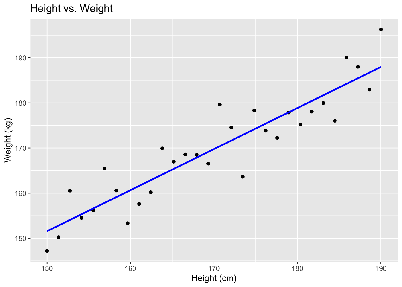
3.4.1 Scatter plot Example

Below is an example of scatter plot depicting a positive association between height and weight.

Code

# set seed for reproducibility
set.seed(123)

# create positively associated example data
height <- seq(150, 190, length.out = 30)
weight <- height + rnorm(30, mean = 0, sd = 5)

# create data frame with height and weight
data <- data.frame(height, weight)

# create trendline graph with ggplot2
library(ggplot2)
ggplot(data, aes(x = height, y = weight)) + 
  geom_point() + 
  geom_smooth(method = "lm", se = FALSE, color = "blue") + 
  labs(title = "Height vs. Weight", x = "Height (cm)", y = "Weight (kg)")

`geom_smooth()` using formula = 'y ~ x'

3.5 Correlation vs. Causation

Correlation vs. Causation It is important to note that correlation does not imply causation. Just because two variables are correlated does not necessarily mean one causes the other. There may be other factors that influence the relationship between the two variables.

For example, a study may find a positive correlation between physical activity and cognitive function. However, this does not necessarily mean that physical activity causes cognitive function. There may be other factors, such as genetics or nutrition, that are also influencing cognitive function.

3.6 Strengths and Limitations of Bivariate Correlation

Bivariate correlation analysis has several strengths and limitations that should be considered when interpreting the results of the analysis.

Strengths:

Bivariate correlation analysis is a straightforward method for examining the relationship between two variables.
The correlation coefficient provides a standardized measure of association that can be easily interpreted.
Correlation analysis can identify potential relationships between variables that may be important for further investigation.

Limitations:

Bivariate correlation analysis only examines the relationship between two variables and does not consider the influence of other variables.
Correlation analysis does not provide information about causation.
The Pearson correlation coefficient assumes that the relationship between the two variables is linear and are approximating normality; this, it may not be appropriate for data that do not meet these assumptions.

4 Conducting Bivariate Correlation Analysis

4.1 Data Requirements

Before conducting a bivariate correlation analysis, certain data requirements must be met:

The two analyzed variables must be measured on a continuous scale.
The data must be at least interval level, meaning the intervals between values are equal.
The data should be free of outliers and other influential data points that could bias the analysis results.

4.2 Steps for Conducting Bivariate Correlation Analysis

Check for normality: If correlating two continuous variables (interval or ratio), it is important to check if both variables are normally distributed. This can be done using statistical tests such as the Shapiro-Wilk test or visual inspection using a histogram or a normal probability plot.
Check for outliers: If extreme outliers are present, you must a decision on how to handle it before proceeding with the analysis.
Calculate the correlation coefficient: The correlation coefficient is calculated using a statistical software package such as jamovi, SPSS or R.
Test for statistical significance: After calculating the correlation coefficient, it is important to test whether the correlation is statistically significant. This can be done by conducting a hypothesis test, typically using a significance level of 0.05.
Interpret the results: After conducting the analysis and determining the significance of the correlation coefficient, it is important to interpret the results. This involves looking at the magnitude and direction of the correlation coefficient and interpreting what it means in the context of the research question.

4.2.1 Example

To illustrate the steps for conducting bivariate Pearson’s correlation analysis, consider a study examining the relationship between exercise intensity and heart rate. The data for this study consists of exercise intensity and heart rate measurements for 50 participants.

Check for normality: Assume that the exercise intensity and heart rate variables are normally distributed after conducting a normality test, which may include graphical visualizations (e.g., histogram and QQ-plots) and more objective measures (e.g., Shapiro-Wilk test, skewness, and kurtosis).
Calculate the correlation coefficient: The correlation coefficient between exercise intensity and heart rate is calculated using Pearson’s correlation coefficient, r = 0.80.
Test for statistical significance: A hypothesis test is conducted to test the significance of the correlation coefficient. The null hypothesis is that the correlation coefficient equals zero, and the alternative hypothesis is that the correlation coefficient does not equal zero. Using a significance level of 0.05, the test indicates that the correlation is statistically significant (p < 0.05).
Interpret the results: The correlation coefficient of 0.80 indicates a strong positive relationship between exercise intensity and heart rate. This means that as exercise intensity increases, heart rate also increases. This finding may have important implications for individuals trying to improve their cardiovascular health through exercise.

5 Hypothesis Testing in Bivariate Correlation Analysis

Bivariate correlation analysis involves hypothesis testing to determine if there is a significant correlation between the variables of interest. Hypothesis testing determines the probability that the correlation coefficient calculated from the sample data is statistically significant, indicating that it is unlikely to have occurred by chance.

The null hypothesis for a bivariate correlation analysis is that there is no significant correlation between the two variables. The alternative hypothesis is that there is a significant correlation between the two variables. The significance level, denoted by α, is the probability of rejecting the null hypothesis when it is true. Common significance levels include 0.05 and 0.01, which correspond to rejecting the null hypothesis when the probability of observing the results by chance is less than 5% or 1%, respectively.

5.1 Stating the null and alternative hypotheses

Follow the example below when stating the null (\(H_0\)) and alternative (\(H_a\)) hypotheses.

\(H_0\): There is no linear correlation between the two variables, or the correlation coefficient is zero.

\(H_1\): There is a linear correlation between the two variables, or the correlation coefficient is not zero.

Mathematically, we can represent the null and alternative hypotheses as:

\(H_0: \rho = 0\)

\(H_1: \rho \neq 0\)

where \(\rho\) is the population correlation coefficient.

To conduct hypothesis testing for a bivariate correlation analysis, the following steps are typically taken:

5.2 Steps

Calculate the correlation coefficient (\(r\)) using the sample data. The correlation coefficient ranges from -1 to 1, with -1 indicating a perfect negative correlation, 1 indicating a perfect positive correlation, and 0 indicating no correlation.
Determine the degrees of freedom (df) equal to the sample size minus two (two variables). Degrees of freedom represent the number of independent observations used to calculate the correlation coefficient.
Use a table or statistical software to determine the critical value of \(r\) for the given significance level (i.e., alpha = 0.05) and degrees of freedom. The critical value of \(r\) represents the value the correlation coefficient must exceed to reject the null hypothesis.
Compare the calculated correlation coefficient to the critical value. If the calculated correlation coefficient is greater than the critical value, reject the null hypothesis and conclude that there is a significant correlation between the two variables. Conversely, if the calculated correlation coefficient is less than the critical value, fail to reject the null hypothesis and conclude that there is no significant correlation between the two variables.

Note

It is important to note that the correlation of two interval (or ratio) variables assumes that the data meet the assumptions of normality and linearity. Normality refers to the assumption that the distribution of the variables being studied is approximately normal. In contrast, linearity is the assumption that the relationship between the two variables is linear. If these assumptions are not met, it may be necessary to use non-parametric correlation coefficients (see Table 1) or transform the data to meet these assumptions.

Additionally, it is important to interpret the results of hypothesis testing in the context of the research question and consider other factors that may influence the relationship between the variables. For example, controlling for confounding variables or conducting subgroup analyses to explore potential interactions may be necessary.

6 Statistical Applications

6.1 jamovi

I will demonstrate how to run the Pearson’s r correlation coefficient below using the esci module (calin-jageman2022?) in jamovi (thejamoviproject2022?).

7 Conclusion

Bivariate correlation analysis is a powerful statistical tool examining the relationship between two continuous variables. While there are assumptions and limitations when using bivariate correlation analysis, it remains useful for Kinesiology researchers to explore various relationships between physical activity, body composition, exercise, and health outcomes. Understanding the data requirements, steps for conducting the analysis, and interpreting the results are essential for utilizing bivariate correlation analysis in Kinesiology research.

Reuse

CC BY-NC 4.0

Citation

BibTeX citation:

@misc{furtado2023,
  author = {Furtado, Ovande},
  title = {Bivariate {Correlation} {Analysis} in {Kinesiology}
    {Research}},
  pages = {undefined},
  date = {2023-03-08},
  url = {https://drfurtado.github.io/randomstats/posts/03062023-bivariate-correlation/},
  langid = {en}
}

For attribution, please cite this work as:

Furtado, O. (2023, March 8). Bivariate Correlation Analysis in Kinesiology Research. RandomStats, undefined. https://drfurtado.github.io/randomstats/posts/03062023-bivariate-correlation/