KIN 610: Quantitative Methods in Kinesiology

Chapter 13: Comparing Two Means

Ovande Furtado Jr., PhD.

Professor, Cal State Northridge

2026-03-04

FYI

This presentation is based on the following books. The references are coming from these books unless otherwise specified.

Main sources:

• Moore, D. S., Notz, W. I., & Fligner, M. (2021). The basic practice of statistics (9th ed.). W.H. Freeman.
• Field, A. (2018). Discovering statistics using IBM SPSS statistics (5th ed.). SAGE Publications.
• Furtado, O., Jr. (2026). Statistics for movement science: A hands-on guide with SPSS (1st ed.). https://drfurtado.github.io/sms

ClassShare App

You may be asked in class to go to the ClassShare App to answer questions.

• https://classsharedrfurtado.netlify.app/

SPSS Tutorial

• SPSS Tutorial: Comparing Two Means

Intro Question

• A researcher measures VO₂max (mL/kg/min) in 25 collegiate athletes and 25 recreationally active non-athletes. Why can’t we just look at the raw sample means to declare the athletes “fitter”? How do we test this statistically?

Click to reveal answer

Simply comparing raw sample means ignores uncertainty and the inherent variability of the data. We need to know whether the observed differences are large enough to infer that true population differences exist, or whether they could plausibly have arisen through sampling variability alone. A t-test quantifies the strength of evidence comparing our two subsets of data against the null hypothesis.

• T-tests account for sample size and data variability, yielding p-values that quantify the strength of evidence.
• We must distinguish between independent samples (two separate groups) and paired samples (comparing two measurements on the same individuals).
• Effect sizes and confidence intervals contextualize our p-values for clear, practical reporting.

Learning Objectives

By the end of this chapter, you should be able to:

• Distinguish between one-sample, independent, and paired sample designs and select the appropriate t-test.
• Conduct and interpret one-sample t-tests for comparing a sample mean to a benchmark.
• Conduct and interpret independent t-tests for comparing two separate groups.
• Conduct and interpret paired t-tests for comparing two related measurements.
• Check assumptions (normality, independence, equal variances) before running formal tests.
• Understand why Welch’s t-test is widely preferred over the pooled-variance t-test.
• Compute and interpret Cohen’s d effect sizes.
• Use confidence intervals to assess the magnitude and precision of mean differences.
• Understand the relationship between sample size, statistical power, and effect detection.
• Evaluate both statistical significance and practical importance of group differences.

Symbols

Symbol	Name	Pronunciation	Definition
\(\bar{x}\)	Sample Mean	“x bar”	Average of a specific sample
\(\mu\)	Population Mean	“mu”	True mean in the entire population
\(\mu_0\)	Hypothesized Mean	“mu zero”	The benchmark value or population constant
\(t\)	T-statistic	“t”	Standardized value representing the difference between groups
\(df\)	Degrees of Freedom	“d - f”	Number of independent values that can vary in your test (\(n-1\) or \(n_1 + n_2 - 2\))
\(\text{SE}_{\text{diff}}\)	Standard Error of the Difference	“S - E diff”	Variability in differences between means given repeated sampling
\(d\)	Cohen’s d	“d”	Standardized effect size quantifying the magnitude of a mean difference
\(n\)	Sample Size	“n”	Number of observations or pairs in a study
\(\alpha\)	Alpha level	“\(\alpha\)”	The significance level (probability of making a Type I error)
\(1 - \beta\)	Statistical Power	“power”	Probability of detecting a true effect when it exists

The Logic of the T-Test

Comparing means between groups or conditions is one of the most fundamental tasks in Movement Science research^[1,2].

Whether evaluating the effectiveness of a training intervention or assessing changes from pre-test to post-test, the t-test provides a principled statistical framework for determining if observed differences are real or just noise^[3].

\[ t = \frac{\text{Observed difference between sample means}}{\text{Standard error of the difference}} \]

• The numerator represents the signal: how far apart are the two groups?
• The denominator represents the noise: how much variability exists in the data across samples?

If the signal is substantially larger than the noise (a large t-value), the p-value will be small, allowing us to reject the null hypothesis^[4].

Three Key Designs

• One-sample samples: One group compared to a constant (e.g., sample mean vs. national average)
• Independent samples: Two separate, unrelated groups (e.g., experimental vs. control)
• Paired samples: Same participants measured twice (e.g., pre-test vs. post-test)

• Emphasize that comparing raw means without accounting for variability is meaningless.
• The t-test asks: “Is the observed difference so large that it’s unlikely to be due to chance?”

One-Sample T-Test: The Basics

A one-sample t-test compares the mean of a single group to a known constant or hypothesized population mean (\(\mu_0\))^[1,3].

When To Use It:

• You have one group of participants and one continuous measurement.
• You want to compare the group mean to a benchmark (e.g., a “passing” score, a neutral point, or a national average).
• The population standard deviation (\(\sigma\)) is unknown^[2].

Key Principle: There is only one group being evaluated against a fixed reference value rather than another group.

Hypotheses Formulation:

Null hypothesis (H₀): \[ \mu = \mu_0 \] The population mean is equal to the benchmark (no difference).

Alternative hypothesis (H₁, two-tailed): \[ \mu \neq \mu_0 \] The population mean differs from the benchmark.

Real Example: Daily Step Count

A researcher measures the average daily step count of 50 students to see if it differs significantly from the recommended target of 10,000 steps. Since one group is compared to a constant, a one-sample t-test is used^[1].

• Clarify that \(\mu_0\) is a fixed number (the “test value”).
• Stress that we use “t” (not “z”) because we usually don’t know the true population \(\sigma\).

Test Statistic Formulation (One-Sample)

The one-sample t-test determines how many standard errors the sample mean is from the hypothesized mean^[1].

\[ t = \frac{\bar{x} - \mu_0}{\text{SE}} \qquad \text{where} \qquad \text{SE} = \frac{s}{\sqrt{n}} \]

Key Components:

• \(\bar{x}\): Sample mean
• \(\mu_0\): Hypothesized population mean (the benchmark)
• \(s\): Sample standard deviation
• \(n\): Sample size
• Degrees of freedom: \(df = n - 1\)

Assumptions:

1. Independence: Each participant’s score is independent of others.
2. Normality: The dependent variable is roughly normally distributed in the population (or \(n\) is large).

SPSS: One-Sample T-Test

In SPSS, go to Analyze → Compare Means → One-Sample T Test. Enter the Test Value (the \(\mu_0\)). See the SPSS Tutorial: One-Sample T-Test.

Worked Example: One-Sample T-Test

A researcher investigates whether the average heart rate of 20 yoga practitioners (\(M = 56.4\) bpm, \(SD = 4.8\)) differs from a target resting heart rate of 60 bpm.

Steps for analysis:

1. State hypotheses:
   • H₀: μ = 60 (heart rate is 60 bpm)
   • H₁: μ ≠ 60 (heart rate differs from 60 bpm)
2. Check assumptions: Evaluate independence and check for normality (Shapiro-Wilk \(p > .05\)).
3. Run the analysis: Input data into SPSS with a Test Value of 60.
4. Interpret results: \(t(19) = -3.35\), \(p = .003\), \(d = -0.75\), 95% CI \([-5.8, -1.4]\) bpm.
5. Report (APA): “The average heart rate of yoga practitioners (\(M = 56.4\) bpm, \(SD = 4.8, n = 20\)) was significantly lower than the target resting heart rate of 60 bpm, \(t(19) = -3.35\), \(p = .003\), \(d = -0.75\).”

• The negative t-value indicates the sample mean is lower than the test value.
• \(d\) is calculated as \((M - \mu_0) / SD\).

Independent Samples: The Basics

An independent samples t-test (two-sample t-test) compares the means of two separate, unrelated groups^[1,3].

When To Use It:

• You have two separate groups (e.g., males vs. females, trained vs. untrained, experimental vs. control).
• Participants are randomly assigned to groups or naturally fall into groups.
• Each participant contributes one score to one group only^[2].

Key Principle: Observations in one group are independent of observations in the other. Knowing the values in Group 1 tells you nothing about the values in Group 2.

Hypotheses Formulation:

Null hypothesis (H₀): \[ \mu_1 = \mu_2 \quad \text{or} \quad \mu_1 - \mu_2 = 0 \] The population means are equal (no difference between groups).

Alternative hypothesis (H₁, two-tailed): \[ \mu_1 \neq \mu_2 \quad \text{or} \quad \mu_1 - \mu_2 \neq 0 \] The population means are not equal (groups differ).

Real Example: Comparing VO₂max

A researcher measures VO₂max (mL/kg/min) in 25 collegiate athletes and 25 recreationally active non-athletes. Since these are two separate, independent groups, an independent t-test is appropriate^[2].

• Ensure students understand what “independent” means: each participant is in ONE group only.
• Two-tailed tests are preferred in most research contexts unless a strong directional prediction exists.

Test Statistic Formulation (Independent)

The independent t-test relies on computing the Standard Error of the difference (\(\text{SE}_{\text{diff}}\)). How we compute this depends on our assumptions about group variances^[5].

1. Equal Variances Assumed (Pooled)

If \(\sigma_1^2 = \sigma_2^2\) (homogeneity of variance), we pool the variances^[3]:

\[ s_p^2 = \frac{(n_1 - 1)s_1^2 + (n_2 - 1)s_2^2}{n_1 + n_2 - 2} \]

\[ \text{SE}_{\text{diff}} = \sqrt{s_p^2 \left(\frac{1}{n_1} + \frac{1}{n_2}\right)} \]

Degrees of freedom: \(df = n_1 + n_2 - 2\)

2. Equal Variances Not Assumed (Welch’s)

If variances differ, use Welch’s t-test^[6]:

\[ \text{SE}_{\text{diff}} = \sqrt{\frac{s_1^2}{n_1} + \frac{s_2^2}{n_2}} \]

Degrees of freedom: (Welch-Satterthwaite approximation) \[ df \approx \frac{\left(\frac{s_1^2}{n_1} + \frac{s_2^2}{n_2}\right)^2}{\frac{(s_1^2/n_1)^2}{n_1-1} + \frac{(s_2^2/n_2)^2}{n_2-1}} \]

Best Practice: Use Welch’s T-Test by Default

Welch’s t-test is more robust and does not require the equal variance assumption. It performs well even when variances are equal, making it a safer default choice^[5,7].

Assumptions of Independent T-Tests

Before computing p-values, we must verify that the dataset meets the necessary statistical assumptions^[1,8].

Assumption	How to check	What to do if violated
1. Independence	Validated via research design (scores in one group cannot influence another).	Use a different statistical model (e.g., paired t-test if actually repeated measures).
2. Normality	Data in both groups should be roughly normally distributed. Check visually (Q-Q plots, histograms) or via Shapiro-Wilk test.	Use data transformations (e.g., log) or nonparametric alternative (Mann-Whitney U). Note: T-tests are robust to non-normality with large samples (N > 30) due to the Central Limit Theorem[9].
3. Homogeneity of Variance	Population variances should be roughly equal. Check via Levene’s test in SPSS.	If Levene’s test \(p < .05\), default to using Welch’s t-test (equal variances not assumed row).

SPSS: Assumptions Check

SPSS reports Levene’s Test for Equality of Variances alongside the t-test output automatically. See the SPSS Tutorial: Checking Assumptions for step-by-step procedures.

• The CLT makes t-tests robust with large samples even if data are non-normal.
• Levene’s p < .05 → use “Equal variances not assumed” (Welch’s) row.

Check Question

You are analyzing reaction times among 14 young adults and 14 older adults. Levene’s Test returns an F-statistic with p = .023. Should you rely on the “Equal variances assumed” row in your SPSS output or the “Equal variances not assumed” row?

Click to reveal answer

Answer: Equal variances not assumed (Welch’s). Because the p-value for Levene’s Test (.023) is below the typical .05 \(\alpha\) threshold, you reject the null hypothesis that variances are equal. The separate variance estimate (Welch’s) must be used. In SPSS, read the “Equal variances not assumed” row for your t-statistic, df, and p-value.

Worked Example: Independent T-Test

A study compares reaction time (ms) between two groups: young adults (\(n=20\), \(M=285\) ms, \(SD=42\)) and older adults (\(n=18\), \(M=342\) ms, \(SD=61\)).

Steps for analysis:

1. State hypotheses:
   • H₀: μ₁ = μ₂ (no difference in reaction time)
   • H₁: μ₁ ≠ μ₂ (reaction times differ)
2. Check assumptions: Evaluate independence, assess normality (Shapiro-Wilk, histograms), check homogeneity of variance (Levene’s test).
3. Run the analysis: SPSS computes the t-statistic, degrees of freedom (Welch-Satterthwaite adjustment), and p-value.
4. Interpret: \(t(29.4) = -3.71\), \(p = .001\), \(d = -1.10\), 95% CI \([-88.4, -25.7]\) ms. Young adults had significantly faster reaction times.
5. Report (APA): “Young adults (\(M = 285.0\) ms, \(SD = 42.0\)) demonstrated significantly faster reaction times than older adults (\(M = 342.0\) ms, \(SD = 61.0\)), \(t(29.4) = -3.71\), \(p = .001\), \(d = -1.10\).”

Calculate in SPSS

See the SPSS Tutorial: Independent-Samples T-Test for step-by-step instructions on running this analysis and interpreting the output.

• Walk through each step carefully — this mirrors the workflow students will follow in labs.
• Point out where each value appears in SPSS output.

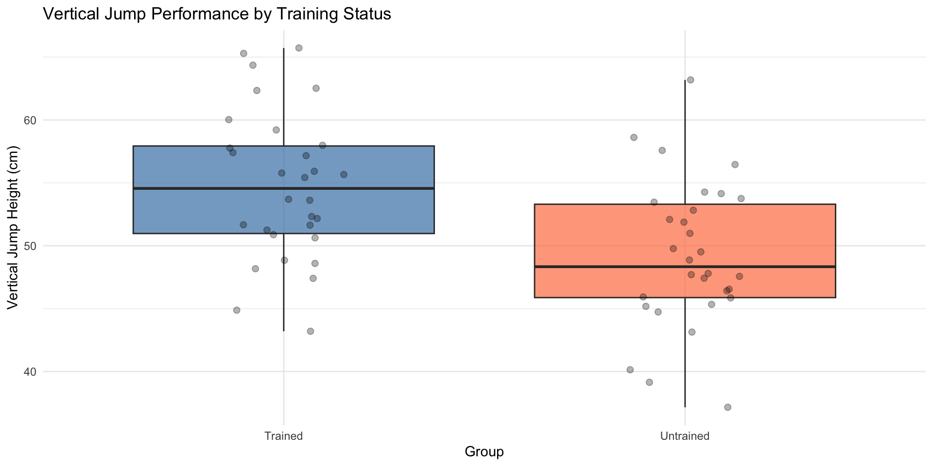
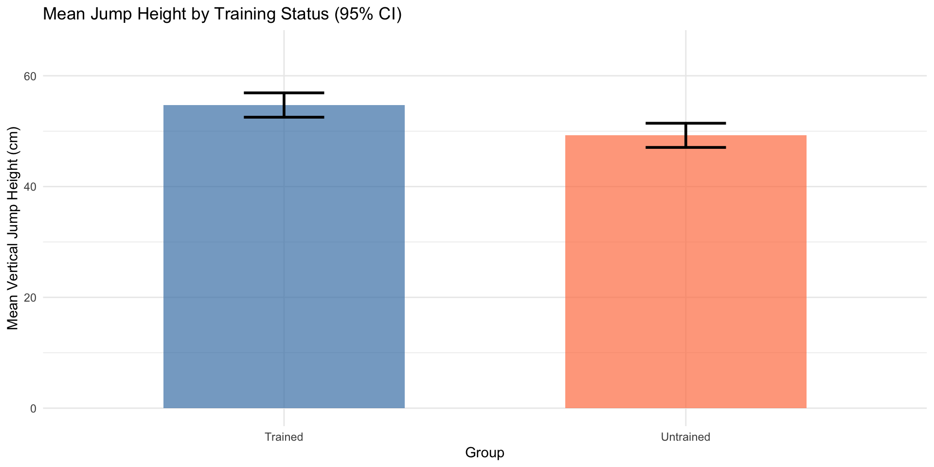
Visualizing Group Comparisons (Independent)

Effective visualizations communicate both central tendency and variability^[10,11].

Figure 1: Comparison of vertical jump height (cm) between trained and untrained groups. Trained athletes demonstrate higher and less variable performance.

Figure 2: Mean vertical jump height with 95% confidence intervals. Non-overlapping error bars suggest a statistically significant difference.

• Box plots reveal distribution shapes, medians, and outliers.
• Non-overlapping 95% CIs suggest roughly p < .01 — but always run the formal test!

Paired Samples: The Basics

A paired samples t-test (dependent/repeated measures t-test) compares two related measurements on the same participants^[1,8].

When To Use It:

• The same participants are measured twice (e.g., pre-test vs. post-test).
• Participants are matched in pairs (twins, left vs. right limbs).
• You want to compare within-subject changes or differences^[12].

Why Paired Designs Are More Powerful: Paired designs control for individual differences by comparing each person to themselves. This removes between-subject variability from the error term, dramatically increasing statistical power^[10,13].

Hypotheses Formulation:

Let \(d_i = x_{i,\text{after}} - x_{i,\text{before}}\) be the difference score for participant \(i\).

Null hypothesis (H₀): \[ \mu_d = 0 \] The mean difference is zero (no change).

Alternative hypothesis (H₁, two-tailed): \[ \mu_d \neq 0 \] The mean difference is not zero (a change occurred).

Real Example: Pre-Post Training Study

A researcher measures vertical jump height in 15 athletes before and after an 8-week plyometric training program. Since the same athletes are measured twice, a paired t-test is appropriate^[2].

• Emphasize the critical distinction: same participants measured twice vs. two separate groups.
• Misclassifying design leads directly to the wrong test.

Test Statistic Formulation (Paired)

The paired t-test is mathematically equivalent to a one-sample t-test on the difference scores^[1]:

\[ t = \frac{\bar{d} - 0}{\text{SE}_d} = \frac{\bar{d}}{s_d / \sqrt{n}} \]

Where: * \(\bar{d}\) = mean of the difference scores * \(s_d\) = standard deviation of the difference scores * \(n\) = number of pairs * \(df = n - 1\)

Assumptions of the Paired T-Test:

1. Pairs are independent: One pair/person does not influence another.
2. Differences are normally distributed: Check normality of the difference scores (\(d = \text{post} - \text{pre}\)), not the raw pre or post scores separately.
3. No order effects: For repeated measures, counterbalancing or randomization prevents systematic order effects (e.g., fatigue or learning)^[12].

Common mistake: Testing raw scores instead of differences

Always check normality on the difference scores (\(d = \text{post} - \text{pre}\)). The paired t-test analyzes differences, so only their distribution matters^[8].

Worked Example: Paired T-Test

A study measures maximal isometric grip strength (kg) before and after a 6-week forearm strengthening program in 12 recreational climbers (\(M_{\text{pre}} = 41.6\) kg, \(SD = 3.75\); \(M_{\text{post}} = 45.9\) kg, \(SD = 4.40\)).

Steps for analysis:

1. State hypotheses:
   • H₀: μ_d = 0 (no change in grip strength)
   • H₁: μ_d ≠ 0 (grip strength changed)
2. Compute differences: Software calculates \(d = \text{post} - \text{pre}\) scores for each participant.
3. Check assumptions: Pairs are independent; test normality of difference scores (Shapiro-Wilk).
4. Run the analysis: SPSS computes \(\bar{d}\), SE, t-statistic, df, and p-value.
5. Interpret: \(t(11) = 16.91\), \(p < .001\), \(d = 4.87\), 95% CI \([3.77, 4.90]\) kg.

Calculate in SPSS

See the SPSS Tutorial: Paired-Samples T-Test for step-by-step instructions on running this analysis, including how to check assumption of normality of difference scores.

• Point out that SPSS automatically computes difference scores — students don’t need to do this manually.
• The effect size here (d = 4.87) is very large because the SD of differences is small relative to the mean change.

Check Question

A graduate student runs a paired t-test on grip strength data (pre vs. post; n = 12 pairs). SPSS shows t(11) = 2.48, p = .031. The student concludes: “The training program was effective because p < .05.” What critical information is the student missing from their conclusion?

Click to reveal answer

Answer: Effect size and confidence interval. Statistical significance alone tells us the difference is unlikely due to chance, but not whether it is practically important. The student should also report: (1) Cohen’s d to quantify the magnitude of the improvement, and (2) the 95% confidence interval for the mean difference to show the precision of the estimate and the plausible range of the true effect. A statistically significant result with d = 0.2 may be trivially small in practice^[4,14].

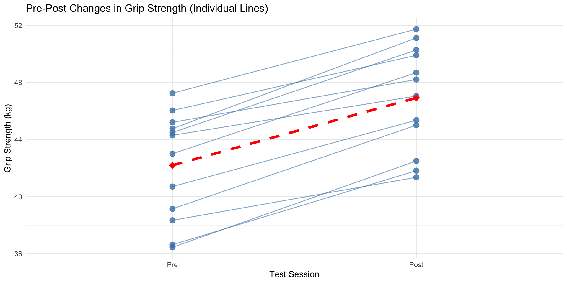
Visualizing Paired Data

For paired data, plotting two disconnected bar charts hides the individual-level changes the test analyzes. Use individual trajectory plots instead^[10].

Why Trajectory Plots?

• Each line traces one participant’s individual change from pre to post.
• You can immediately spot outliers or sub-groups (e.g., responders vs. non-responders).
• The red dashed line shows the mean change — directly mapping to the paired t-test result.
• Reveals within-subject vs. between-subject variability clearly.

Figure 3: Individual changes in grip strength (kg) from pre-test to post-test. Each line represents one participant. Red dashed line = mean change.

• In Fig 13.3, all lines slope upward — strong evidence of a consistent improvement across participants.
• One or two flat or downward-sloping lines would suggest non-responders worth investigating.

Effect Sizes: Cohen’s d

Statistical significance (\(p < \alpha\)) tells us whether an effect is detectable — effect sizes tell us how large it is, and are essential for evaluating practical importance^[15,16].

Cohen’s d is the gold-standard standardized effect size for mean differences:

\[ d = \frac{\bar{x}_1 - \bar{x}_2}{s_{\text{pooled}}} \quad \text{(Independent)} \qquad d = \frac{\bar{d}}{s_d} \quad \text{(Paired)} \]

Benchmarks (Cohen, 1988):

\(|d|\)	Interpretation
0.2	Small effect
0.5	Medium effect
0.8	Large effect

Context is Crucial

Cohen’s benchmarks are guidelines, not absolute rules^[16]. A “small” effect (\(d = 0.2\)) may save lives in injury prevention research. In elite athletics, even a “large” effect may be unrealistic. Always interpret relative to your research domain^[14,17].

Modern SPSS (v27) computes Cohen’s d and its confidence intervals automatically when you check Estimate effect sizes — no manual calculation needed.

• Emphasize: p-value = detection; effect size = magnitude.
• SPSS now outputs d directly — students don’t need to calculate by hand.

Confidence Intervals for Mean Differences

P-values only tell us whether an effect exists. Confidence intervals (CIs) tell us how large it is and how precisely we’ve estimated it^[4].

What CIs tell you:

• Significance: If the CI for the difference does not include zero → statistically significant.

  • 95% CI [0.5, 8.2] cm → significant, but wide (uncertain)
  • 95% CI [4.0, 4.8] cm → significant, and narrow (precise)

• Practical Importance: Are the plausible effect magnitudes meaningful in practice?

• Width reflects precision: Narrow CIs → large samples, low variability. Wide CIs → small samples, high variability.

Statistical vs. Practical Significance:

	Statistical	Practical
Question	Is the effect real?	Does it matter?
Tool	p-value	Effect size (\(d\)), CI
Risk	Large \(n\) → small trivial effects become “significant”	Small effect may still be important in clinical contexts

Always Report Both!

A statistically significant result with \(d = 0.05\) and \(n = 10{,}000\) is practically meaningless^[14,18].

• The CI is the most informative single summary: it combines significance AND precision.
• Wide CI = “we found something, but we don’t know how big it is.”

Check Question

A study reports that an 8-week training program improved vertical jump height. The independent t-test result is: t(38) = 2.12, p = .041, 95% CI [0.2, 5.8] cm, d = 0.67. Which statement is most accurate?

Click to reveal answer

Answer: The effect is statistically significant with a medium effect size, but the CI is wide, indicating uncertainty about the true magnitude. The 95% CI [0.2, 5.8] cm excludes zero (significant at α = .05), and d = 0.67 suggests a medium effect. However, the wide CI means the true population difference could range from a trivial 0.2 cm to a meaningful 5.8 cm — so while statistically significant, we need larger samples to precisely estimate the practical magnitude^[4].

Sample Size and Statistical Power

Statistical power (\(1 - \beta\)) is the probability of detecting a true effect when it actually exists^[13,15]. Underpowered studies produce false negatives — missing real effects and wasting resources.

Factors affecting Statistical Power:

1. Sample size (\(n\)): Larger \(n\) → higher power
2. Effect size (\(d\)): Larger effects are easier to detect
3. Significance level (\(\alpha\)): Higher \(\alpha\) → higher power (but more Type I error risk)
4. Variability (\(s\)): Less “noisy” data yields higher power
5. Research Design: Paired designs have much higher power than independent (they control for individual differences)^[13]

Recommended Target: Power ≥ 0.80 (80%) — a conventional minimum^[15].

A Priori vs. Post Hoc:

Type	When	Purpose
A Priori	Before data collection	Determine required sample size for desired power (use G*Power)
Post Hoc	After data collection	Avoid! Mathematically circular — non-significant results always yield low observed power by definition[19]

Use G*Power for Sample Size Planning

**G*Power** is free software for power analysis. Input your expected effect size (\(d\)), desired power (.80), and α (.05) to determine required \(n\). Available at psychologie.hhu.de.

• Post hoc power is circular: if p > .05, observed power will always be low. Report CI width instead.
• G*Power is free, easy, and the standard tool for reporting sample size justification.

Comparing Two Proportions (Z-Test)

T-tests compare means of continuous variables. For proportions (e.g., injury rates, success rates, proportions), we use the two-proportion z-test^[1,20].

For proportions \(p_1\) and \(p_2\), the test statistic is:

\[ z = \frac{p_1 - p_2}{\text{SE}_{\text{diff}}} \]

Where the standard error uses separate proportions (for CIs): \[ \text{SE}_{\text{diff}} = \sqrt{\frac{p_1(1-p_1)}{n_1} + \frac{p_2(1-p_2)}{n_2}} \]

For large samples, \(z\) follows the standard normal distribution.

Real Example: Injury Rates

A study finds 18 of 100 runners using minimalist shoes (18%) suffered injuries, compared to 12 of 100 using traditional shoes (12%). A two-proportion z-test yields \(z = 1.20\), \(p = .23\), suggesting no significant difference in injury rates^[20].

Pooled vs. Unpooled SE

For significance testing under H₀: \(p_1 = p_2\), software uses the pooled proportion \(\hat{p} = (x_1x_2)/(n_1n_2)\). Both approaches give similar results with large samples^[20].

Common Misconceptions

Misconception 1

❌ Incorrect: “p < .05 means the effect is large and important.”

✅ Correct: Statistical significance only tells you the effect is unlikely due to chance. With very large samples, even trivially small effects (e.g., \(d = 0.02\)) can reach significance. Always report effect sizes and CIs to assess practical importance^[14,18].

Misconception 2

❌ Incorrect: “My data are non-normal, so I can’t run a t-test.”

✅ Correct: T-tests are robust to non-normality with large samples (n > 30) due to the Central Limit Theorem^[9]. For small samples, check normality carefully; nonparametric alternatives are available if severely violated^[8].

Misconception 3

❌ Incorrect: “I should use an independent t-test for my pre-post study since I’m comparing two time points.”

✅ Correct: Pre-post data on the same participants require a paired t-test. Using an independent t-test ignores the within-subject correlations, wastes statistical power, and produces incorrect results^[2,13].

Misconception 4

❌ Incorrect: “Non-significant means there’s no difference.”

✅ Correct: Non-significance means insufficient evidence given this sample to reject H₀. A small, underpowered study may miss a real effect entirely. Report the CI width — a wide CI spanning both meaningful and trivial values means the study was underpowered, not that no difference exists^[4,21].

• Misconceptions 1 and 4 are extremely common in student lab reports.
• Misconception 3 is the core design error — mispairing data is among the most important practical mistakes.

Independent vs. Paired: Which Test?

Use this decision table when designing your analysis^[2,12]:

Characteristic	One-Sample T-Test	Independent T-Test	Paired T-Test
Design	One group vs. benchmark	Two separate groups	Same participants measured twice (or matched pairs)
Assumptions	Independence, normality	Independence, normality per group, (equal variances)	Pairs independent, difference scores normally distributed
Power	N/A	Lower (between-subject variability in error)	Higher (controls for individual differences)
Example	Average steps vs. 10k target	Trained vs. untrained athletes	Athletes measured pre- and post-training
Null hypothesis	\(\mu = \mu_0\)	\(\mu_1 = \mu_2\)	\(\mu_d = 0\)
Degrees of freedom	\(n - 1\)	\(n_1 + n_2 - 2\) (or Welch’s df)	\(n - 1\) (n = number of pairs)

Critical Design Error

Using an independent t-test when data are truly paired loses all the power advantage of the paired design. Always match the test to the research design, not to how data happen to be arranged in SPSS^[8,13].

When T-Tests Fail: Nonparametric Alternatives

Non-parametric tests make fewer assumptions about the underlying distribution of the data^[22].

Key Characteristics:

• Distribution-free: Do not require the data to follow a normal distribution.
• Rank-based: Typically rely on ranks or medians instead of means and standard deviations.
• Robust: More robust when data are skewed, contain outliers, or when sample sizes are small^[22].

Common Comparisons:

Goal	Parametric Test	Nonparametric Alternative
One Group vs. Constant	One-Sample t-test	Wilcoxon Signed-Rank
Two Independent Groups	Independent t-test	Mann-Whitney U
Two Related Samples	Paired t-test	Wilcoxon Signed-Rank

Power Trade-off

Non-parametric tests usually have less statistical power than parametric tests when assumptions hold. Use them as alternatives when assumptions cannot be justified^[8].

• These tests are sometimes called “distribution-free” because they don’t assume a normal curve.
• They are particularly useful for small samples (n < 30) where the Central Limit Theorem doesn’t protect the t-test from skewness.
• They “rank” the data (1st, 2nd, 3rd…) rather than using the raw values.

Workflow Summary

Use this sequence whenever you compare means between two groups or conditions^[1,8]:

Step	Action	Tool/Check
1	Identify the research design	One-sample, independent, or paired?
2	State hypotheses	H₀: no difference; H₁: difference exists
3	Screen your data	Histograms, Q-Q plots, boxplots
4	Check assumptions	Normality (Shapiro-Wilk), independence, Levene’s test (for independent)
5	Select and run the test	One-Sample, Independent, or Paired T-Test in SPSS with Estimate effect sizes checked
6	Calculate effect size	Cohen’s \(d\) (auto-output by SPSS v27)
7	Interpret results	p-value + CI + \(d\) together
8	Report transparently (APA)	M, SD, n, \(t\), df, \(p\), CI, \(d\)

The Goal Is Not Just Numbers

Always ask: “Is the observed difference statistically detectable (p-value)? Is it practically important (effect size)? How precisely have we estimated it (confidence interval)?”

Reporting T-Tests in APA Style

APA-style reporting includes: descriptive statistics, test statistic, df, exact p-value, CI, and effect size^[11,23].

One-Sample T-Test Template:

“The [sample] (\(M\) = [mean], \(SD\) = [SD], \(n\) = [n]) [differed/did not differ] significantly from the [benchmark/population mean] of [value], \(t\)([df]) = [t-value], \(p\) = [p-value], \(d\) = [Cohen’s d], 95% CI [lower, upper].”

“The average heart rate (\(M = 56.4\) bpm, \(SD = 4.8, n = 20\)) was significantly lower than the target heart rate of 60 bpm, \(t(19) = -3.35\), \(p = .003\), \(d = -0.75\).”

Independent T-Test Template:

“[Group 1] (\(M\) = [mean], \(SD\) = [SD], \(n\) = [n]) [differed/did not differ] significantly from [Group 2] (\(M\) = [mean], \(SD\) = [SD], \(n\) = [n]), \(t\)([df]) = [t-value], \(p\) = [p-value], \(d\) = [Cohen’s d], 95% CI [lower, upper].”

“Trained athletes (\(M = 55.3\) cm, \(SD = 6.2\), \(n = 30\)) demonstrated significantly higher vertical jump performance than untrained controls (\(M = 47.8\) cm, \(SD = 7.1\), \(n = 30\)), \(t\)(58) = 4.52, \(p < .001\), \(d = 1.12\), 95% CI [4.2, 10.8] cm.”

Paired T-Test Template:

“[Condition 2] (\(M\) = [mean], \(SD\) = [SD]) was significantly [higher/lower] than [Condition 1] (\(M\) = [mean], \(SD\) = [SD]), \(t\)([df]) = [t-value], \(p\) = [p-value], mean difference = [M_diff], 95% CI [lower, upper], \(d\) = [Cohen’s d].”

“Post-training grip strength (\(M = 45.9\) kg, \(SD = 4.40\)) was significantly greater than pre-training strength (\(M = 41.6\) kg, \(SD = 3.75\)), \(t\)(11) = 16.91, \(p < .001\), mean difference = 4.3 kg, 95% CI [3.77, 4.90], \(d = 4.87\).”

SPSS: APA Reporting

See the SPSS Tutorial: Reporting Guidelines for full write-up examples and formatting tips for lab reports.

Key Takeaways

1. T-tests compare means between groups or conditions; choose one-sample (vs. benchmark), independent (separate groups), or paired (same participants) based strictly on research design.
2. Welch’s t-test is the recommended default for independent designs — it handles unequal variances without penalty when variances are equal.
3. Assumptions matter: Check normality and Levene’s test; use nonparametric alternatives (Mann-Whitney U, Wilcoxon) when severely violated.
4. Cohen’s d quantifies practical magnitude. SPSS v27 outputs it automatically with “Estimate effect sizes” checked.
5. Confidence intervals are more informative than p-values alone — they show the size and precision of the difference.
6. Statistical ≠ Practical significance: A significant p-value does not guarantee a meaningful effect.
7. Plot your data before testing: box plots (independent) and trajectory plots (paired) reveal what numbers alone cannot.
8. Power matters: Aim for ≥ 0.80 power via a priori sample size planning (G*Power).

Core Principle

Always ask: “Is the effect detectable (p)? How large is it (d)? How precisely estimated (CI)? Does it matter in practice?”

Practice Questions

1. A researcher compares the average BMI of 50 local seniors to the national average of 26.5. Which t-test is appropriate and why?
2. A researcher measures balance scores in 20 yoga practitioners and 20 sedentary adults. Which t-test is appropriate and why?
3. A pre-post study tests grip strength in 15 participants before and after a training program. Which t-test is appropriate and why?
4. SPSS output shows Levene’s \(F = 4.82\), \(p = .034\). Which row should you read for the t-test results?
5. A study finds \(t(28) = 2.11\), \(p = .044\), \(d = 0.38\). Interpret both statistical and practical significance.
6. Why is reporting only “p = .03” insufficient in an APA results section?
7. A student checks normality on the pre- and post-test scores separately before a paired t-test. What is wrong with this approach?
8. Explain why a paired t-test typically has more statistical power than an independent t-test with the same number of observations.
9. A 95% CI for the mean difference is [−0.8, 5.2] cm. What can you conclude about statistical significance and practical significance?

Exit Ticket: Comparing Two Means Activity

Your instructor will provide you with a link to the activity in Canvas

References

1. Moore, D. S., McCabe, G. P., & Craig, B. A. (2021). Introduction to the practice of statistics (10th ed.). W. H. Freeman; Company.

2. Weir, J. P., & Vincent, W. J. (2021). Statistics in kinesiology (5th ed.). Human Kinetics.

3. Student [Gosset, W. S. (1908). The probable error of a mean. Biometrika, 6(1), 1–25. https://doi.org/10.2307/2331554

4. Cumming, G. (2014). The new statistics: Why and how. Psychological Science, 25(1), 7–29. https://doi.org/10.1177/0956797613504966

5. Delacre, M., Lakens, D., & Leys, C. (2017). Why psychologists should by default use welch’s t-test instead of student’s t-test. International Review of Social Psychology, 30(1), 92–101. https://doi.org/10.5334/irsp.82

6. Welch, B. L. (1947). The generalization of "student’s" problem when several different population variances are involved. Biometrika, 34(1-2), 28–35. https://doi.org/10.1093/biomet/34.1-2.28

7. Ruxton, G. D. (2006). The unequal variance t-test is an underused alternative to student’s t-test and the mann-whitney u test. Behavioral Ecology, 17(4), 688–690. https://doi.org/10.1093/beheco/ark016

8. Field, A. (2018). Discovering statistics using IBM SPSS statistics (5th ed.). SAGE Publications.

9. Lumley, T., Diehr, P., Emerson, S., & Chen, L. (2002). The importance of the normality assumption in large public health data sets. Annual Review of Public Health, 23, 151–169. https://doi.org/10.1146/annurev.publhealth.23.100901.140546

10. Cumming, G. (2012). Understanding the new statistics: Effect sizes, confidence intervals, and meta-analysis. Routledge.

11. Wilkinson, L., & Task Force on Statistical Inference. (1999). Statistical methods in psychology journals: Guidelines and explanations. American Psychologist, 54(8), 594–604. https://doi.org/10.1037/0003-066X.54.8.594

12. Thomas, L. (2015). How to estimate power and sample size. Trauma Surgery & Acute Care Open, 1(1), e000005. https://doi.org/10.1136/tsaco-2015-000005

13. Maxwell, S. E., Delaney, H. D., & Kelley, K. (2018). Designing experiments and analyzing data: A model comparison perspective (3rd ed.). Routledge.

14. Batterham, A. M., & Hopkins, W. G. (2006). Making meaningful inferences about magnitudes. International Journal of Sports Physiology and Performance, 1(1), 50–57. https://doi.org/10.1123/ijspp.1.1.50

15. Cohen, J. (1988). Statistical power analysis for the behavioral sciences (2nd ed.). Lawrence Erlbaum Associates.

16. Lakens, D. (2013). Calculating and reporting effect sizes to facilitate cumulative science: A practical primer for t-tests and ANOVAs. Frontiers in Psychology, 4, 863. https://doi.org/10.3389/fpsyg.2013.00863

17. Hopkins, W. G. (2000). Measures of reliability in sports medicine and science. Sports Medicine, 30(1), 1–15. https://doi.org/10.2165/00007256-200030010-00001

18. Cohen, J. (1994). The earth is round (p < .05). American Psychologist, 49(12), 997–1003. https://doi.org/10.1037/0003-066X.49.12.997

19. Hoenig, J. M., & Heisey, D. M. (2001). ABCs of alpha, beta, delta, and epsilon. Ecology, 82(12), 3369–3372. https://doi.org/10.1890/0012-9658(2001)082[3369:AOABDE]2.0.CO;2

20. Agresti, A. (2003). Categorical data analysis.

21. Altman, D. G., & Bland, J. M. (1995). Statistics notes: Absence of evidence is not evidence of absence. BMJ, 311, 485. https://doi.org/10.1136/bmj.311.7003.485

22. Conover, W. J. (1999). Practical nonparametric statistics.

23. American Psychological Association. (2020). Publication manual of the american psychological association (7th ed.). American Psychological Association.

24. Furtado, O., Jr. (2026). Statistics for movement science: A hands-on guide with SPSS (1st ed.). https://drfurtado.github.io/sms/