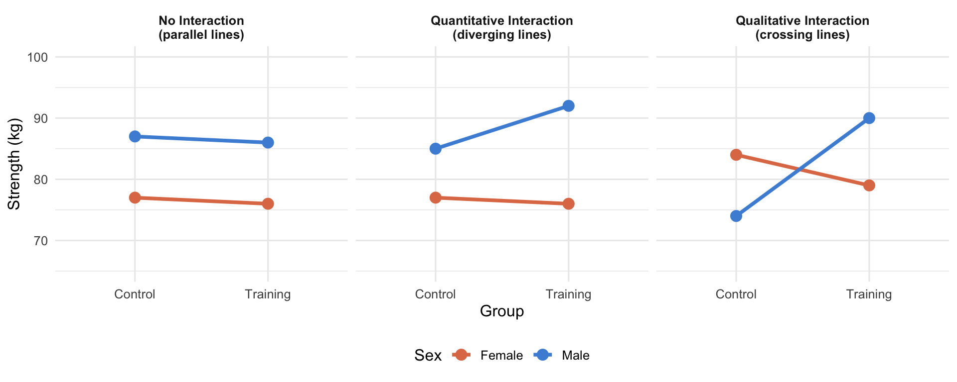
Within-Within Factorial ANOVA
Both factors are evaluated as repeated-measures, meaning ALL participants complete EVERY combination of levels.
A 2 × 2 Within-Within Design (4 conditions per person):
| Rested |
Rested-Morning |
Rested-Evening |
| Fatigued |
Fatigued-Morning |
Fatigued-Evening |
Variance and Error Terms: - Three distinct error terms are calculated! - Factor A has its own error term (\(SS_{A \times Subjects}\)). - Factor B has its own error term (\(SS_{B \times Subjects}\)). - The Interaction has its own error term (\(SS_{A \times B \times Subjects}\)).
Because the same participants complete all conditions, individual subject differences are completely removed from all error terms, making this an extremely high-powered design.
Effect Sizes for Factorial ANOVA
Partial eta-squared (η²_p) is reported by SPSS for every effect:
\[\eta^2_p = \frac{SS_{\text{effect}}}{SS_{\text{effect}} + SS_{\text{error}}}\]
The “error” changes by effect in a mixed ANOVA:
| Group |
\(SS_{\text{Subjects/Group}}\) (between-subjects error) |
| Time |
\(SS_{\text{Time × Subjects/Group}}\) (within-subjects error) |
| Group × Time |
\(SS_{\text{Time × Subjects/Group}}\) (within-subjects error) |
Partial omega-squared (ω²_p) — less biased, recommended for small-to-moderate samples:
\[\omega^2_p = \frac{SS_{\text{effect}} - df_{\text{effect}} \cdot MS_{\text{error}}}{SS_{\text{effect}} + (N \cdot p - df_{\text{effect}}) \cdot MS_{\text{error}}}\]
Cohen’s benchmarks (small ≈ .01, medium ≈ .06, large ≥ .14) apply cautiously — well-controlled lab training studies routinely produce η²_p > .50 for within-subjects effects.
Report η²_p AND ω²_p for every source, not only the “significant” ones. Readers need all values to evaluate power and practical significance.
APA Reporting Template
For a mixed ANOVA with a significant interaction:
“A 2 ([Factor A levels]) × [k] ([Factor B levels]) mixed ANOVA was conducted with [DV] as the dependent variable. Mauchly’s test indicated that the sphericity assumption [was/was not] violated, W([df]) = [W], p = [p]. [Correction applied (ε = value) if violated.] The [Factor A × Factor B] interaction was [significant/not significant], F([df1], [df2]) = [F], p = [p], η²_p = [value], ω²_p = [value]. [Simple effects follow-up.] The main effect of [Factor B] was [significant], F([df1], [df2]) = [F], p = [p], η²_p = [value], ω²_p = [value]. The main effect of [Factor A] was [not significant], F([df1], [df2]) = [F], p = [p], η²_p = [value].”
Full example (Group × Time):
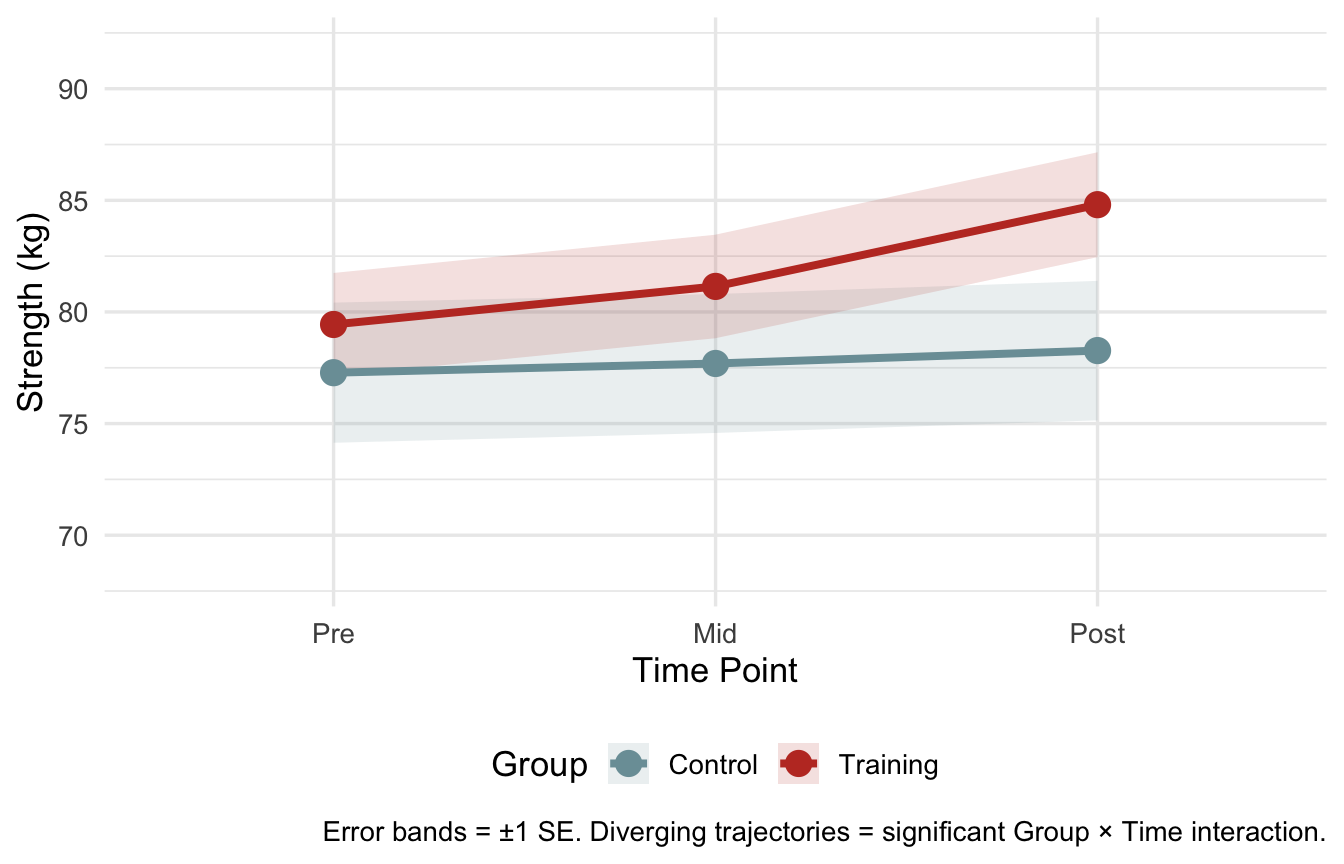
“A 2 (Group: control, training) × 3 (Time: pre, mid, post) mixed ANOVA was conducted with strength (kg) as the dependent variable. Mauchly’s test indicated that the sphericity assumption was not violated, W(2) = .93, p = .059. The Group × Time interaction was statistically significant, F(2, 116) = 61.00, p < .001, η²_p = .51, ω²_p = .40, indicating that the two groups followed different strength trajectories over 12 weeks. Simple effects analysis revealed a significant effect of Time within the training group, with progressive gains from pre (M = 79.67 kg) to post (M = 85.06 kg), while Time was not significant within the control group. The main effect of Time was significant, F(2, 116) = 108.55, p < .001, η²_p = .65, ω²_p = .54. The main effect of Group was not significant, F(1, 58) = 2.52, p = .117, η²_p = .04.”