KIN 610: Quantitative Methods in Kinesiology

Chapter 15: Analysis of Variance With Repeated Measures

Ovande Furtado Jr., PhD.

Professor, Cal State Northridge

2026-04-14

FYI

This presentation is based on the following books. The references are coming from these books unless otherwise specified.

Main sources:

• Weir, J. P., & Vincent, W. J. (2021). Statistics in kinesiology (5th ed.). Human Kinetics.
• Field, A. (2018). Discovering statistics using IBM SPSS statistics (5th ed.). SAGE Publications.
• Furtado, O., Jr. (2026). Statistics for movement science: A hands-on guide with SPSS (1st ed.). https://drfurtado.github.io/sms

ClassShare App

You may be asked in class to go to the ClassShare App to answer questions.

• https://classshare-b44e7.web.app/

SPSS Tutorial

• SPSS Tutorial: Repeated Measures ANOVA

Intro Question

• A physical therapist measures balance error scores in 25 older adults at three time points: before a 12-week fall-prevention program (pre), at 6 weeks (mid), and at 12 weeks (post). She wants to know whether balance improved over the program. Why is a between-subjects ANOVA not appropriate here, and what should she use instead?

Click to reveal answer

A between-subjects ANOVA is inappropriate because the same participants are measured at all three time points — the observations are not independent across conditions, and treating them as such would ignore the correlation among repeated measurements. The correct approach is a one-way repeated measures ANOVA, which partitions out between-subjects variability (individual differences in baseline balance) from the error term, producing a much more sensitive test of the time effect.

• Repeated measures designs measure the same participants under all conditions or time points.
• The key advantage is removing individual differences from the error term — participants serve as their own controls.
• One-way repeated measures ANOVA extends the paired t-test to three or more conditions while controlling the familywise error rate.

Learning Objectives

By the end of this chapter, you should be able to:

• Explain why repeated measures designs offer greater statistical power than equivalent between-subjects designs
• Describe how total variance is partitioned in a one-way repeated measures ANOVA
• State the sphericity assumption and explain its meaning in plain language
• Interpret Mauchly’s test and select the appropriate degrees-of-freedom correction
• Conduct and interpret Bonferroni-corrected pairwise comparisons after a significant omnibus F
• Compute and interpret partial eta-squared (η²_p) and partial omega-squared (ω²_p)
• Report a complete one-way repeated measures ANOVA in APA format

Symbols

Symbol	Name	Pronunciation	Definition
\(SS_{BS}\)	Between-subjects SS	“SS between subjects”	Variance due to consistent individual differences
\(SS_{time}\)	Time SS	“SS time”	Variance due to the within-subjects factor
\(SS_{error}\)	Error SS	“SS error”	Subjects × time interaction (within-subject inconsistency)
\(W\)	Mauchly’s W	“W”	Test statistic for the sphericity assumption
\(\varepsilon\)	Epsilon	“epsilon”	Degree of sphericity (1.0 = perfect; lower = more violated)
\(\hat{\varepsilon}_{GG}\)	Greenhouse-Geisser epsilon	“GG epsilon”	Conservative df correction factor
\(\tilde{\varepsilon}_{HF}\)	Huynh-Feldt epsilon	“HF epsilon”	Less conservative df correction factor
\(\eta^2_p\)	Partial eta-squared	“partial eta squared”	Time effect relative to within-subject error
\(\omega^2_p\)	Partial omega-squared	“partial omega squared”	Less-biased estimate of population partial effect size

Within-Subject vs. Between-Subject Designs

Between-subjects design (Chapter 14):

• Each participant appears in one group only
• Individual differences (genetics, baseline fitness) remain in the error term
• Error = true treatment effect + individual variability
• Requires more participants to achieve adequate power

Within-subjects (repeated measures) design:

• The same participants appear in all conditions
• Each participant’s consistent baseline level cancels out across conditions
• Error = only the inconsistency in how participants respond differently across time
• Result: much smaller error term → larger F → greater power

Intuition: Imagine measuring grip strength pre, mid, and post training.

• Participant A (athlete) starts at 110 kg, ends at 118 kg
• Participant B (sedentary) starts at 60 kg, ends at 67 kg

A between-subjects design treats the 50 kg baseline gap as error. A repeated measures design asks: “Relative to each person’s own starting point, how much did they change?” The baseline gap disappears — only the ~7–8 kg change is analyzed.

• Use the grip strength example to ground the statistical logic in something tangible.
• Emphasize that within-subjects error is NOT the same as within-groups error from between-subjects ANOVA.

Partitioning Variance in Repeated Measures ANOVA

In a between-subjects ANOVA, total variance splits two ways:

\[SS_{\text{total}} = SS_{\text{between groups}} + SS_{\text{within groups}}\]

The F-ratio = \(MS_{\text{between groups}} / MS_{\text{within groups}}\), and individual differences inflate the denominator.

In a one-way repeated measures ANOVA, a third split is possible:

\[SS_{\text{total}} = SS_{\text{between subjects}} + SS_{\text{time}} + SS_{\text{error}}\]

Source	What it captures	In F-ratio?
\(SS_{\text{between subjects}}\)	Consistent individual differences (some people always score higher)	Removed from denominator
\(SS_{\text{time}}\)	How means change across time points — the effect we want	Numerator (\(MS_{\text{time}}\))
\(SS_{\text{error}}\)	How differently each participant responds across time (subjects × time)	Denominator (\(MS_{\text{error}}\))

Because \(SS_{\text{between subjects}}\) is removed, \(MS_{\text{error}}\) is much smaller → \(F\) is larger for the same treatment effect.

• Draw a diagram if possible: total variance split into 3 pieces, with the between-subjects piece “grayed out” from the F calculation.

Hypotheses and When to Use Repeated Measures ANOVA

Use one-way repeated measures ANOVA when:

• The same participants provide data at three or more time points or conditions
• The outcome variable is continuous
• Every participant contributes exactly one observation at each level of the factor
• The goal is to test whether population means differ across conditions

Hypotheses:

\[H_0: \mu_{\text{pre}} = \mu_{\text{mid}} = \mu_{\text{post}}\]

Time has no effect on the dependent variable — population means are equal at all time points.

\[H_1: \text{At least one population mean differs from the others}\]

Connection to simpler tests

• Two time points only? → Use the paired t-test (equivalent to repeated measures ANOVA with \(k = 2\))
• Ordinal outcome or severe non-normality with small n? → Use Friedman’s ANOVA by ranks (Ch. 19)

• Remind students: a significant omnibus F only tells you somewhere there is a difference — post hoc tests reveal which pairs differ.

Assumptions of One-Way Repeated Measures ANOVA

Three assumptions must be met:

1. Independence of participants — Scores from different participants must be unrelated to one another. By contrast, repeated scores from the same participant are expected to be related because the design tracks within-person change over time. This assumption is handled by the study design, not fixed statistically afterward.

2. Normality of difference scores — Unlike between-subjects ANOVA (which requires normality of raw scores), repeated measures ANOVA requires that the pairwise differences (e.g., mid − pre, post − pre, post − mid) are approximately normally distributed. Check with histograms, Q-Q plots, and Shapiro-Wilk tests on the difference scores. Robust to mild violations when \(n \geq 30\).

3. Sphericity — The variances of all pairwise difference scores must be approximately equal. This is the most distinctive and frequently violated assumption — checked with Mauchly’s test.

Sphericity ≠ Homogeneity of Variance

A common misconception: sphericity does not require equal variances of the raw scores. It requires equal variances of the pairwise differences. A dataset can have unequal SDs at pre, mid, and post and still satisfy sphericity if the changes are consistent across individuals.

The Sphericity Assumption

Sphericity requires that the variances of the differences between all pairs of time points are approximately equal:

\[\text{Var}(\text{mid} - \text{pre}) \approx \text{Var}(\text{post} - \text{pre}) \approx \text{Var}(\text{post} - \text{mid})\]

Why it matters:

• The standard repeated measures F-test assumes homogeneous pairwise difference variances when computing degrees of freedom
• When sphericity is violated, the df are too large → the test is anticonservative → inflated Type I error
• In practice: you reject H₀ more often than your stated α level

Plain language: Sphericity is violated when some time intervals produce highly variable change (some participants improve a lot, others barely at all) while other intervals produce very uniform change (everyone improves about the same amount).

Sphericity with only two time points

When there are only two levels, sphericity cannot be violated — a single difference score has only one variance, so the assumption is automatically satisfied. Mauchly’s test is grayed out or absent in SPSS output for two-level factors.

Mauchly’s Test of Sphericity

SPSS automatically reports Mauchly’s W when you run a repeated measures ANOVA.

Mauchly’s W	Interpretation
W = 1.0	Perfect sphericity
0 < W < 1	Departures from sphericity

Decision rule:

Mauchly’s p	Action
p > .05	Sphericity not rejected → use “Sphericity Assumed” row
p < .05	Sphericity violated → apply a degrees-of-freedom correction

Epsilon (ε) estimates quantify the severity of the violation:

• Range: \(\frac{1}{k-1}\) (complete non-sphericity) to 1.0 (perfect sphericity)
• For 3 time points: minimum possible ε = .50
• ε close to 1.0 → minor violation; ε far below 1.0 → serious violation

Sample size sensitivity

Mauchly’s test is sensitive to sample size: small samples may miss real violations; large samples may flag trivial ones. Always inspect epsilon alongside the p-value. An ε ≥ .90 suggests approximate sphericity even if Mauchly’s p < .05 in a large sample.

Sphericity Corrections: GG and HF

When Mauchly’s p < .05, reduce the df by multiplying by epsilon:

\[df_{\text{corrected}} = df \times \hat{\varepsilon}\]

The F-statistic itself does not change — only the df and resulting p-value change.

Greenhouse-Geisser (GG): Conservative correction using \(\hat{\varepsilon}_{GG}\). Tends to overcorrect (reduces power) when ε > .75.

Huynh-Feldt (HF): Less conservative correction using \(\tilde{\varepsilon}_{HF}\) (always ≥ \(\hat{\varepsilon}_{GG}\)). Better balance of error control and power when violation is moderate.

Decision rule (Girden, 1992):

GG Epsilon	Use
\(\hat{\varepsilon}_{GG} \geq .75\)	Huynh-Feldt correction
\(\hat{\varepsilon}_{GG} < .75\)	Greenhouse-Geisser correction
Mauchly’s p > .05	Sphericity Assumed (no correction)

Tip

Always report the correction used and the epsilon value in your APA write-up so readers can evaluate your decision.

• Walk students through an example: df = 2 and 58, ε_GG = .78. Corrected df = 1.56 and 45.24. F stays the same; p changes.

Worked Example: Strength Across a 12-Week Program

Thirty university students had muscular strength (kg) measured at pre, mid (6-week), and post (12-week) of a resistance training program.

Descriptive statistics:

Time Point	n	M (kg)	SD
Pre-training	30	79.7	12.3
Mid-training (6-week)	30	81.7	12.3
Post-training (12-week)	30	85.1	12.5

Mauchly’s test: W(2) = .932, p = .054 → sphericity not violated → use Sphericity Assumed row.

ANOVA source table:

Source	SS	df	MS	F	p	η²_p
Time	443.73	2	221.87	116.0	< .001	.80
Error (Time)	110.94	58	1.91
Participants	13,120.63	29

Conclusion: F(2, 58) = 116.0, p < .001, η²_p = .80 — a statistically significant and very large effect of training time on muscular strength.

How to read η²_p = .80

Partial eta-squared of .80 means that, after removing between-subject differences, about 80% of the within-subject variance is associated with time.

Common benchmark standards for η²_p are often attributed to Cohen^[1] and discussed in modern reporting guidance by Lakens^[2]:

• .01 = small
• .06 = medium
• .14 = large

So η²_p = .80 is not just large by the usual standard, it is an extremely large effect.

Post Hoc Tests for Repeated Measures ANOVA

A significant omnibus F tells you that somewhere across the time points there is a meaningful change — but not which pairs differ.

Bonferroni-corrected pairwise comparisons are recommended^[3]:

• Adjusts the significance threshold for the number of comparisons
• For 3 time points: 3 possible pairs (pre vs. mid, pre vs. post, mid vs. post)
• In SPSS: Estimated Marginal Means → Options → Bonferroni

Results from strength training example:

Comparison	Mean Difference (kg)	SE	p (adjusted)	95% CI
Mid − Pre	2.02	0.27	< .001	[1.34, 2.70]
Post − Pre	5.38	0.33	< .001	[4.54, 6.22]
Post − Mid	3.36	0.45	< .001	[2.22, 4.50]

All three pairwise comparisons were significant: strength increased progressively and significantly at each stage.

Only after a significant omnibus F

Never run post hoc pairwise comparisons following a non-significant overall F-test. Doing so inflates Type I error.

Effect Sizes: Partial Eta-Squared and Partial Omega-Squared

Partial eta-squared (η²_p) — reported by SPSS:

\[\eta^2_p = \frac{SS_{\text{time}}}{SS_{\text{time}} + SS_{\text{error}}}\]

Note: \(SS_{\text{between subjects}}\) is excluded from the denominator.

Cohen’s (1988) benchmarks:

η²_p	Interpretation
.01	Small
.06	Medium
.14	Large

Strength example: η²_p = .80 (very large — 80% of within-subject variance is explained by time).

Partial omega-squared (ω²_p) — less biased, not computed by SPSS directly:

\[\omega^2_p = \frac{(k-1)(MS_{\text{time}} - MS_{\text{error}})}{(k-1) \cdot MS_{\text{time}} + (n - k + 1) \cdot MS_{\text{error}}}\]

Strength example:

\[\omega^2_p = \frac{(2)(221.87 - 1.91)}{(2)(221.87) + (29)(1.91)} = \frac{439.92}{499.13} \approx .88\]

ω²_p corrects for the upward bias in η²_p — recommended for small-to-moderate samples.

η²_p > full η²

Partial eta-squared excludes between-subjects variance from the denominator, so it is typically larger than full η². Always label it as partial and do not compare it directly with η² from between-subjects studies.

Visualizing Repeated Measures Results

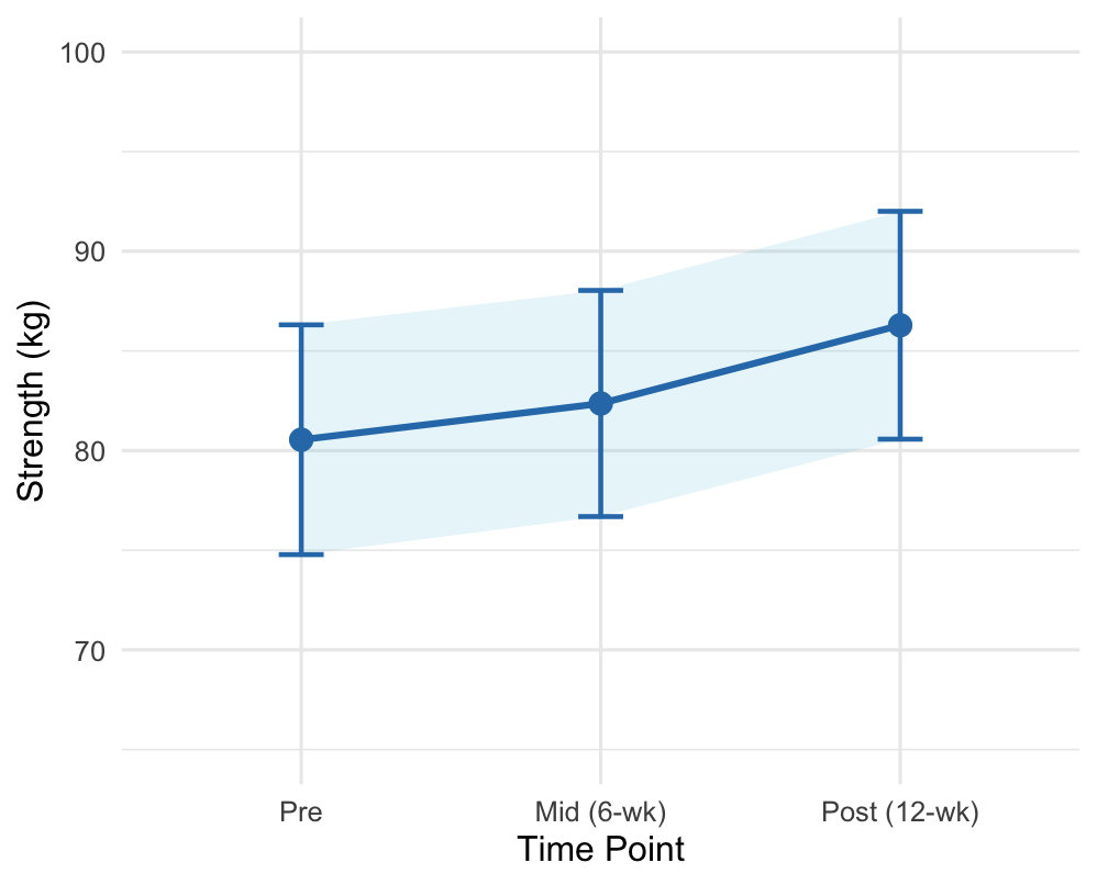
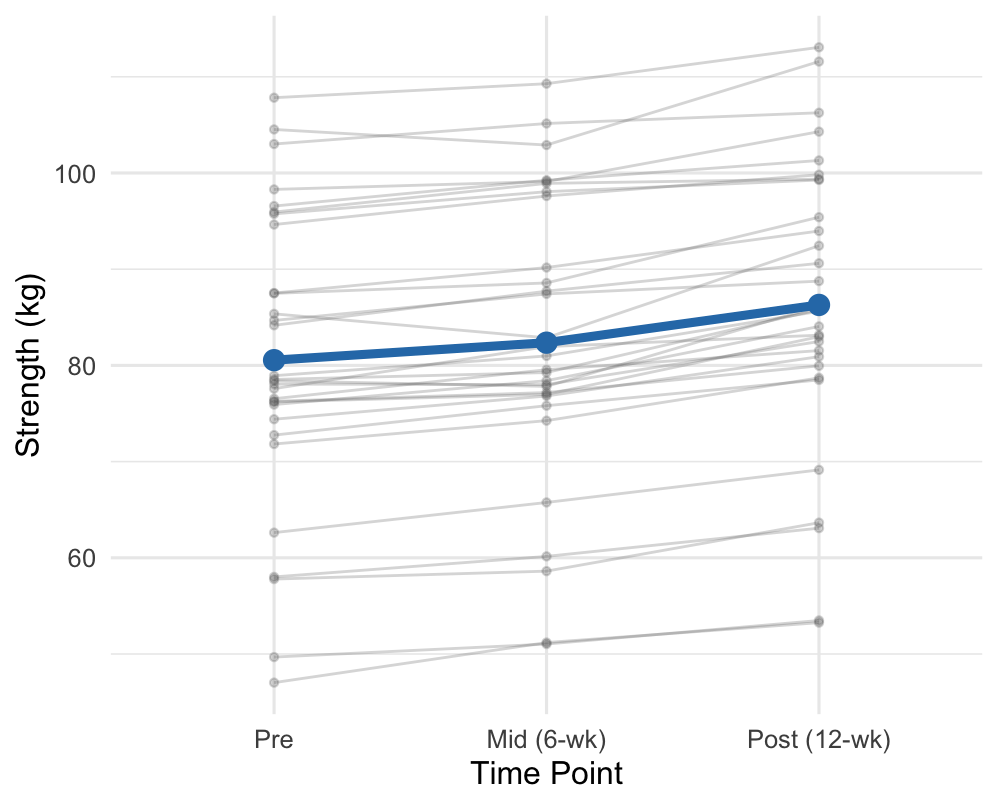
Two recommended plots for within-subject data:

Line plot with error bars:

• X-axis: time points (pre, mid, post)
• Y-axis: group mean of the outcome
• Error bars: 95% confidence intervals
• Non-overlapping CIs indicate statistically significant and practically meaningful differences

Best for: showing the overall group trajectory and precision of estimates.

Figure 1

Spaghetti plot:

• Each thin line = one participant’s trajectory
• Bold line = group mean
• Lines moving predominantly in the same direction → consistent within-subject effect, small error, high power
• Lines that cross or reverse → inconsistent responses, larger error variance, lower power

Best for: revealing individual-level consistency and evaluating whether the error term is likely to be small.

Figure 2

• Emphasize the spaghetti plot as a diagnostic tool — if lines go in all different directions, the error term will be large and power will be lower than expected.

APA Reporting Template

Template:

“A one-way repeated measures ANOVA examined the effect of [factor] on [DV]. Mauchly’s test indicated that the sphericity assumption [was/was not] violated, W([df]) = [W], p = [p]. [Therefore, degrees of freedom were corrected using the [Greenhouse-Geisser/Huynh-Feldt] estimate of sphericity (ε = [value]).] The within-subjects effect of [factor] was [significant/not significant], F([df_time], [df_error]) = [F], p = [p], η²_p = [value], ω²_p = [value]. Post hoc Bonferroni comparisons revealed that [specific pairwise results].”

Full example (strength training data):

“A one-way repeated measures ANOVA was conducted to examine the effect of training time (pre, mid, post) on muscular strength. Mauchly’s test indicated that the sphericity assumption was not violated, W(2) = .932, p = .054. The within-subjects effect of time was statistically significant, F(2, 58) = 116.0, p < .001, η²_p = .80, ω²_p = .88. Post hoc Bonferroni-corrected pairwise comparisons indicated that strength increased significantly from pre- to mid-training (M difference = 2.02 kg, p < .001, 95% CI [1.34, 2.70]), from mid- to post-training (M difference = 3.36 kg, p < .001, 95% CI [2.22, 4.50]), and from pre- to post-training (M difference = 5.38 kg, p < .001, 95% CI [4.54, 6.22]).”

Tip

Always report which correction was used and the epsilon value. Readers need this information to evaluate your analytic decisions and replicate your findings.

Common Pitfalls

1. Ignoring Mauchly’s test and always using “Sphericity Assumed” — When Mauchly’s is significant and ε is notably below 1.0, the uncorrected F-test rejects H₀ too often. Always check Mauchly’s result first and apply GG or HF correction when warranted.

2. Treating η²_p as though it were full η² — Partial eta-squared excludes between-subjects variance from the denominator, making it larger than full η². Always label it as partial and avoid direct comparisons with η² values from between-subjects studies.

3. Running post hoc tests after a non-significant omnibus F — Pairwise comparisons are only justified following a significant F. Running them after a non-significant result capitalizes on chance and inflates Type I error.

4. Confusing within-subjects error with between-subjects error — The error term in repeated measures ANOVA (\(MS_{\text{error}}\) = \(MS_{\text{subjects × time}}\)) reflects individual inconsistency in responses across time points — not total within-group variability. This distinction is essential for correctly reading the SPSS source table.

Check Question

SPSS reports Mauchly’s W = .762, p = .019, ε_GG = .82. Which row in the SPSS Within-Subjects Effects table should you use to report your F-test results, and why?

Click to reveal answer

Answer: Because Mauchly’s p = .019 < .05, the sphericity assumption is violated and you must not use the “Sphericity Assumed” row. Next, check ε_GG = .82, which is ≥ .75. Following Girden’s (1992) decision rule, you should apply the Huynh-Feldt correction — the GG correction would be overly conservative here. Use the Huynh-Feldt row in the SPSS output and report the HF-corrected df, F, and p-value. Remember to report the epsilon value and name the correction in your APA write-up.

Chapter Summary

Key takeaways:

• Repeated measures designs remove between-subjects variance from the error term, producing greater statistical power than equivalent between-subjects designs
• SS partitioning: \(SS_{\text{total}} = SS_{\text{between subjects}} + SS_{\text{time}} + SS_{\text{error}}\); only \(SS_{\text{time}}\) and \(SS_{\text{error}}\) appear in the F-ratio
• Sphericity is the critical and unique assumption: equal variances of pairwise difference scores. Checked with Mauchly’s W
• When sphericity is violated: use GG correction if ε_GG < .75; use HF correction if ε_GG ≥ .75
• Post hoc tests (Bonferroni) are only run after a significant omnibus F
• Report both η²_p (SPSS default) and ω²_p (less biased); always label η²_p as partial
• A complete APA report includes Mauchly’s test, correction used, omnibus F, descriptive statistics, and Bonferroni pairwise comparisons

References

1. Cohen, J. (1988). Statistical power analysis for the behavioral sciences (2nd ed.). Lawrence Erlbaum Associates.

2. Lakens, D. (2013). Calculating and reporting effect sizes to facilitate cumulative science: A practical primer for t-tests and ANOVAs. Frontiers in Psychology, 4, 863. https://doi.org/10.3389/fpsyg.2013.00863

3. Field, A. (2018). Discovering statistics using IBM SPSS statistics (5th ed.). SAGE Publications.

4. Furtado, O., Jr. (2026). Statistics for movement science: A hands-on guide with SPSS (1st ed.). https://drfurtado.github.io/sms/