KIN 610: Quantitative Methods in Kinesiology

Chapter 14: Analysis of Variance

Ovande Furtado Jr., PhD.

Professor, Cal State Northridge

2026-04-07

FYI

This presentation is based on the following books. The references are coming from these books unless otherwise specified.

Main sources:

• Moore, D. S., Notz, W. I., & Fligner, M. (2021). The basic practice of statistics (9th ed.). W.H. Freeman.
• Field, A. (2018). Discovering statistics using IBM SPSS statistics (5th ed.). SAGE Publications.
• Furtado, O., Jr. (2026). Statistics for movement science: A hands-on guide with SPSS (1st ed.). https://drfurtado.github.io/sms

ClassShare App

You may be asked in class to go to the ClassShare App to answer questions.

• https://classshare-b44e7.web.app/

SPSS Tutorial

• SPSS Tutorial: One-Way ANOVA

Intro Question

• A researcher wants to compare VO₂max across three training groups: endurance, resistance, and control. A colleague suggests running three separate t-tests. Why is this approach problematic, and what should be done instead?

Click to reveal answer

Running three t-tests inflates the familywise error rate — the probability of at least one false positive rises from 5% to nearly 14%. Analysis of Variance (ANOVA) tests all group means simultaneously in a single analysis that maintains the stated α level. If the omnibus F is significant, post hoc tests then identify which specific pairs differ while still controlling for multiple comparisons.

• ANOVA controls Type I error when comparing three or more group means.

Learning Objectives

By the end of this chapter, you should be able to:

• Explain why ANOVA is required when comparing three or more groups instead of multiple t-tests.
• Describe how total variance is partitioned into between-groups and within-groups components.
• Construct and interpret an ANOVA source table, including SS, df, MS, F, and p.
• State the null and alternative hypotheses for a one-way ANOVA.
• Check the assumptions of one-way ANOVA (independence, normality, homogeneity of variance).
• Select the appropriate post hoc test based on whether assumptions are met.
• Interpret post hoc comparison output and identify which group pairs differ.
• Compute and interpret effect sizes (η² and ω²) for one-way ANOVA results.
• Report one-way ANOVA results in APA format.

Symbols

Symbol	Name	Pronunciation	Definition
\(\mu\)	Population Mean	“mu”	True mean in the entire population
\(k\)	Number of Groups	“k”	Total number of treatment levels or groups
\(N\)	Total Sample Size	“N”	Total number of observations across all groups
\(SS_B\)	Between-Groups SS	“S-S between”	Sum of squares reflecting variability of group means around the grand mean
\(SS_W\)	Within-Groups SS	“S-S within”	Sum of squares reflecting variability of scores around their group mean
\(MS\)	Mean Square	“M-S”	Variance estimate; SS divided by its degrees of freedom
\(F\)	F-ratio	“F”	Ratio of between-groups to within-groups variance
\(\eta^2\)	Eta-squared	“eta squared”	Proportion of total variance explained by the independent variable
\(\omega^2\)	Omega-squared	“omega squared”	Less biased estimate of the population effect size
\(\alpha\)	Alpha level	“\(\alpha\)”	Significance level (probability of a Type I error)

The Multiple Comparisons Problem

When comparing three or more groups, the temptation is to run pairwise t-tests for every combination^[1,2].

Why multiple t-tests are wrong:

With \(c\) independent comparisons each at \(\alpha = .05\), the familywise error rate is:

\[ \alpha_{\text{FW}} = 1 - (1 - \alpha)^c \]

Groups	Comparisons	Familywise α
3	3	≈ .14
4	6	≈ .26
5	10	≈ .40

The ANOVA solution:

ANOVA tests one omnibus null hypothesis—that all group means are equal—in a single analysis that maintains the stated α^[3].

\[ H_0: \mu_1 = \mu_2 = \mu_3 = \ldots = \mu_k \]

If the omnibus F is significant, post hoc tests then make pairwise comparisons while controlling the familywise error rate.

Never substitute multiple t-tests for ANOVA

Running uncorrected pairwise t-tests when comparing three or more groups is not just a stylistic choice—it is a methodological error that produces misleading conclusions^[1].

• Emphasize that this is not a technicality; inflated Type I error means results cannot be trusted.
• Students often resist this because “t-tests feel familiar.” Reinforce that ANOVA is the correct tool.

The F-Statistic

The F-ratio is the core of ANOVA — a signal-to-noise ratio^[3,4]:

\[ F = \frac{MS_{\text{between}}}{MS_{\text{within}}} = \frac{\text{Signal}}{\text{Noise}} \]

When H₀ is true (all means equal):

Both \(MS_B\) and \(MS_W\) estimate the same population variance.

\[F \approx 1\]

The F-distribution is always positive and right-skewed. Its shape is determined by \((df_B, df_W)\).

When H₁ is true (at least one mean differs):

\(MS_B\) is inflated by real group differences; \(MS_W\) is unaffected.

\[F > 1\]

Large F values are unlikely under H₀ and provide strong evidence to reject it.

What F does NOT tell you

A significant F only tells you that somewhere among the groups a difference exists. It does not tell you which specific pairs of groups differ. Post hoc tests are required for that^[2].

• The F-distribution is always ≥ 0 because it is a ratio of variances.
• Stress: F ≈ 1 under H₀, F > 1 under H₁. We never expect F to be exactly 1 even under H₀ due to sampling variability.

One-Way ANOVA: When to Use It

One-way between-subjects ANOVA is appropriate when^[5–7]:

Design requirements:

1. A single categorical independent variable (factor) with three or more levels
2. A continuous dependent variable (interval or ratio scale)
3. Each participant belongs to one and only one group (between-subjects)
4. Groups consist of different participants

If only two groups: use an independent t-test.

If same participants across conditions: use Repeated Measures ANOVA (Chapter 15).

Movement science examples:

IV (Groups)	DV	Test
Training type (3)	VO₂max	One-way ANOVA
Age category (4)	Balance score	One-way ANOVA
Sport level (3)	Grip strength	One-way ANOVA
Rehab protocol (3)	ROM (degrees)	One-way ANOVA

Real Example: Comparing VO₂max Across Training Groups

A researcher randomly assigns 60 students to one of three 12-week programs: endurance training (n = 20), resistance training (n = 20), or no-exercise control (n = 20). VO₂max is measured at post-training. With one factor (training group) at three levels and a continuous DV, one-way ANOVA is appropriate^[5].

• Common mistake: students use ANOVA for two groups. Reinforce that t-test is for 2 groups, ANOVA for 3+.
• Another common mistake: using one-way ANOVA when the same participants are measured repeatedly. That requires repeated measures ANOVA.

Hypotheses for One-Way ANOVA

Null hypothesis (H₀):

All population group means are equal — the independent variable has no effect on the dependent variable:

\[ H_0: \mu_1 = \mu_2 = \mu_3 = \ldots = \mu_k \]

Alternative hypothesis (H₁):

At least one population mean differs from the others:

\[ H_1: \text{at least one } \mu_j \neq \mu_{j'} \]

Note: H₁ does not specify which groups differ — only that some difference exists somewhere among the means.

Steps for conducting a one-way ANOVA:

Step	Action
1	State H₀ and H₁; set α (typically .05)
2	Check assumptions (independence, normality, homogeneity of variance)
3	Run the ANOVA in SPSS and examine the source table
4	If F is significant, run post hoc tests
5	Compute effect sizes (η² or ω²)
6	Report results in APA format

• The omnibus test is always first. Jumping straight to post hoc tests without a significant F is a methodological error.
• Remind students: with 3 groups there are 3 possible pairs; with 4 groups, 6 pairs; and so on.

Assumptions of One-Way ANOVA

Before computing F, verify three key assumptions^[1,2,4]:

Assumption	How to check	What to do if violated
1. Independence	Validated via research design (random assignment, no repeated measures).	Use a different model (e.g., repeated measures ANOVA for within-subjects designs).
2. Normality	Check within each group separately using histograms, Q-Q plots, and the Shapiro-Wilk test (p > .05 = normal). ANOVA is robust with n ≥ 30 per group due to the CLT[8].	Log/square-root transformations or the nonparametric Kruskal-Wallis test (Chapter 19).
3. Homogeneity of variance	Use Levene’s test (p > .05 = equal variances). Practical rule: largest SD < twice the smallest SD.	Use Welch’s ANOVA or Brown-Forsythe ANOVA; switch post hoc tests to Games-Howell[9,10].

When Levene’s test is significant (p < .05)

Switch from the standard F-test to Welch’s ANOVA (available under Analyze → Compare Means → One-Way ANOVA → Options → Welch). Use Games-Howell instead of Tukey HSD for post hoc comparisons^[2].

• Normality: check each group separately, not the overall pooled distribution.
• Independence is the most critical — it cannot be corrected statistically once violated.
• Levene’s test itself can be sensitive in large samples; the SD rule of thumb is a useful supplement.

Worked Example: One-Way ANOVA

A researcher compares VO₂max (mL·kg⁻¹·min⁻¹) in 60 students randomly assigned to three 12-week programs: endurance (n = 20), resistance (n = 20), and control (n = 20).

Step 1: State hypotheses

• H₀: μ_endurance = μ_resistance = μ_control (training group has no effect on VO₂max)
• H₁: At least one group mean differs; α = .05

Step 2: Check assumptions

Independence confirmed by design; Shapiro-Wilk p > .05 in each group; Levene’s p = .312 (equal variances assumed).

Step 3: Run ANOVA in SPSS; interpret source table

Source	SS	df	MS	F	p
Between groups	1,248.6	2	624.3	14.87	< .001
Within groups	2,391.4	57	41.95
Total	3,640.0	59

With F(2, 57) = 14.87, p < .001, we reject H₀. Post hoc tests are needed to identify which pairs differ.

SPSS: Run One-Way ANOVA

Analyze → Compare Means → One-Way ANOVA. Add DV to Dependent List and grouping variable to Factor. Under Options, check Descriptive and Homogeneity of variance test. See the SPSS Tutorial: One-Way ANOVA.

• Walk through each cell of the source table.
• df_B = 3 − 1 = 2; df_W = 60 − 3 = 57; they sum to df_T = 59. ✓
• MS_B = 1248.6/2 = 624.3; MS_W = 2391.4/57 = 41.95; F = 624.3/41.95 = 14.87. ✓

Check Question

A researcher compares flexibility (degrees) across four age groups (n = 15 per group). Levene’s test returns F(3, 56) = 4.12, p = .011. What should the researcher do?

Click to reveal answer

Answer: Because Levene’s test is significant (p = .011 < .05), the homogeneity of variance assumption is violated. The researcher should use Welch’s ANOVA (or Brown-Forsythe ANOVA) instead of the standard F-test, and apply Games-Howell post hoc comparisons rather than Tukey HSD. In SPSS: Analyze → Compare Means → One-Way ANOVA → Options → check Welch and Brown-Forsythe.

Open the ClassShare App to answer this question:

https://classshare-b44e7.web.app/

Post Hoc Tests: Introduction

A significant F-test tells us something is different — post hoc tests tell us what^[1,11].

Why post hoc tests are needed:

• The omnibus F only establishes that at least one mean differs.
• Post hoc tests make all pairwise comparisons (e.g., Group 1 vs. 2, 1 vs. 3, 2 vs. 3) while controlling the familywise error rate.
• They should only be run after a significant omnibus F.

Never run post hoc tests on a non-significant F

Applying post hoc tests when the omnibus F is not significant — “fishing” — inflates Type I error and produces unreliable conclusions^[2].

Choosing the right post hoc test:

Test	Equal variances?	Best for
Tukey HSD	Yes	Most common; good balance of Type I/II error
Bonferroni	Yes	Small number of comparisons; conservative
Games-Howell	No	When Levene’s is significant
Scheffé	Yes	most conservative

Rule: Use Tukey HSD when assumptions are met. Switch to Games-Howell when Levene’s is significant^[2,10].

• Tukey HSD is the default recommendation for most Movement Science research.
• Bonferroni is more conservative (lower power) and best when the researcher has a small number of specific comparisons in mind.
• Games-Howell is robust and performs well with both equal and unequal group sizes.

Interpreting Post Hoc Output

Following the VO₂max example, Tukey HSD post hoc comparisons reveal which specific pairs differ^[11]:

Comparison	Mean Difference	SE	p (adjusted)†	95% CI
Endurance − Resistance	7.2	2.05	.003	[2.1, 12.3]
Endurance − Control	11.8	2.05	< .001	[6.7, 16.9]
Resistance − Control	4.6	2.05	.082	[−0.5, 9.7]

^† Why “adjusted”? Each individual t-test runs at α = .05. With three comparisons, the chance of at least one false positive rises to ~14%. Tukey HSD corrects each p-value upward so that the risk of any false positive across all comparisons combined stays at .05.

Check Question

Based on the Tukey HSD output below, which training groups differed significantly in VO₂max?

Comparison	Mean Difference	SE	p (adjusted)	95% CI
Endurance − Resistance	7.2	2.05	.003	[2.1, 12.3]
Endurance − Control	11.8	2.05	< .001	[6.7, 16.9]
Resistance − Control	4.6	2.05	.082	[−0.5, 9.7]

Click to reveal answer

Answer: Endurance vs. Resistance (p = .003) and Endurance vs. Control (p < .001) were both significant. Resistance vs. Control (p = .082) was not significant.

Open the ClassShare App to answer this question:

https://classshare-b44e7.web.app/

SPSS: Post Hoc Tests

In the One-Way ANOVA dialog, click Post Hoc. Select Tukey (if equal variances) or Games-Howell (if unequal). See the SPSS Tutorial: Post Hoc Tests.

• Note that 95% CIs that exclude zero = significant at α = .05; CIs that include zero = non-significant.
• The adjusted p-values from Tukey HSD account for all comparisons simultaneously.

Check Question

A one-way ANOVA comparing balance scores across three groups (n = 16 per group, N = 48) produces F(2, 45) = 5.83, p = .006. Levene’s test is non-significant. A student concludes that all three groups differ from each other. Is this conclusion correct?

Hint: df₁ = k − 1 = 3 − 1 = 2 (Between-groups row); df₂ = N − k = 48 − 3 = 45 (Within-groups row)

Click to reveal answer

Answer: No. A significant omnibus F only tells us that at least one group mean differs — it does not specify which pairs. The student must run Tukey HSD post hoc tests (since Levene’s is non-significant) to determine which specific group pairs are significantly different. Some comparisons may be significant and others may not.

Effect Sizes in ANOVA

A significant F-test answers whether groups differ — effect sizes answer how much^[12–14].

Eta-squared (η²)

\[ \eta^2 = \frac{SS_{\text{between}}}{SS_{\text{total}}} \]

• Proportion of total variance explained by the IV
• Simple to compute from source table
• Overestimates population effect, especially with small samples^[15]
• VO₂max example: \(\eta^2 = 1248.6 / 3640.0 = .34\)

Omega-squared (ω²) — preferred for reporting

\[ \omega^2 = \frac{SS_{\text{between}} - (k-1) \cdot MS_{\text{within}}}{SS_{\text{total}} + MS_{\text{within}}} \]

• Less biased estimate of the population effect^[13,15]
• VO₂max: \(\omega^2 = (1248.6 - 2 \times 41.95) / (3640.0 + 41.95) \approx .32\)

Cohen’s (1988) benchmarks (η² and ω²):

Effect	Value
Small	.01
Medium	.06
Large	.14

Report both η² and ω²

Report ω² as the primary effect size; include η² alongside it when comparing to prior literature (which typically reports η²). Always note that η² is upwardly biased^[13,15].

Source	SS	df	MS	F	p
Between groups	1,248.6	2	624.3	14.87	< .001
Within groups	2,391.4	57	41.95
Total	3,640.0	59

Cohen’s f — for power analysis (G*Power):

\[ f = \sqrt{\frac{\eta^2}{1 - \eta^2}} \]

• Convert η² from your ANOVA output and enter f into G*Power to compute achieved power or required N
• VO₂max example: \(f = \sqrt{.34 / .66} \approx .72\) (well above the “large” threshold of .40)

Effect	f
Small	.10
Medium	.25
Large	.40

• η² = R² in regression; ω² = adjusted R² analogy — both measure proportion of variance explained.
• With total N < 100, η² can meaningfully overstate the true effect.
• Cohen’s f is the input G*Power requires for ANOVA power analysis. Convert: f = sqrt(eta2 / (1 - eta2)).

Visualizing ANOVA Results

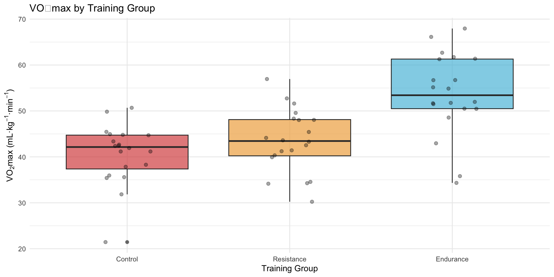
Effective visualizations communicate both central tendency and variability across all groups^[16,17].

Figure 1: VO₂max (mL·kg⁻¹·min⁻¹) across three training groups. Box plots display the median, IQR, and outliers. Endurance training produced notably higher VO₂max values.

Figure 2: Mean VO₂max with 95% confidence intervals. Non-overlapping CIs between endurance and control groups strongly suggest a statistically significant difference.

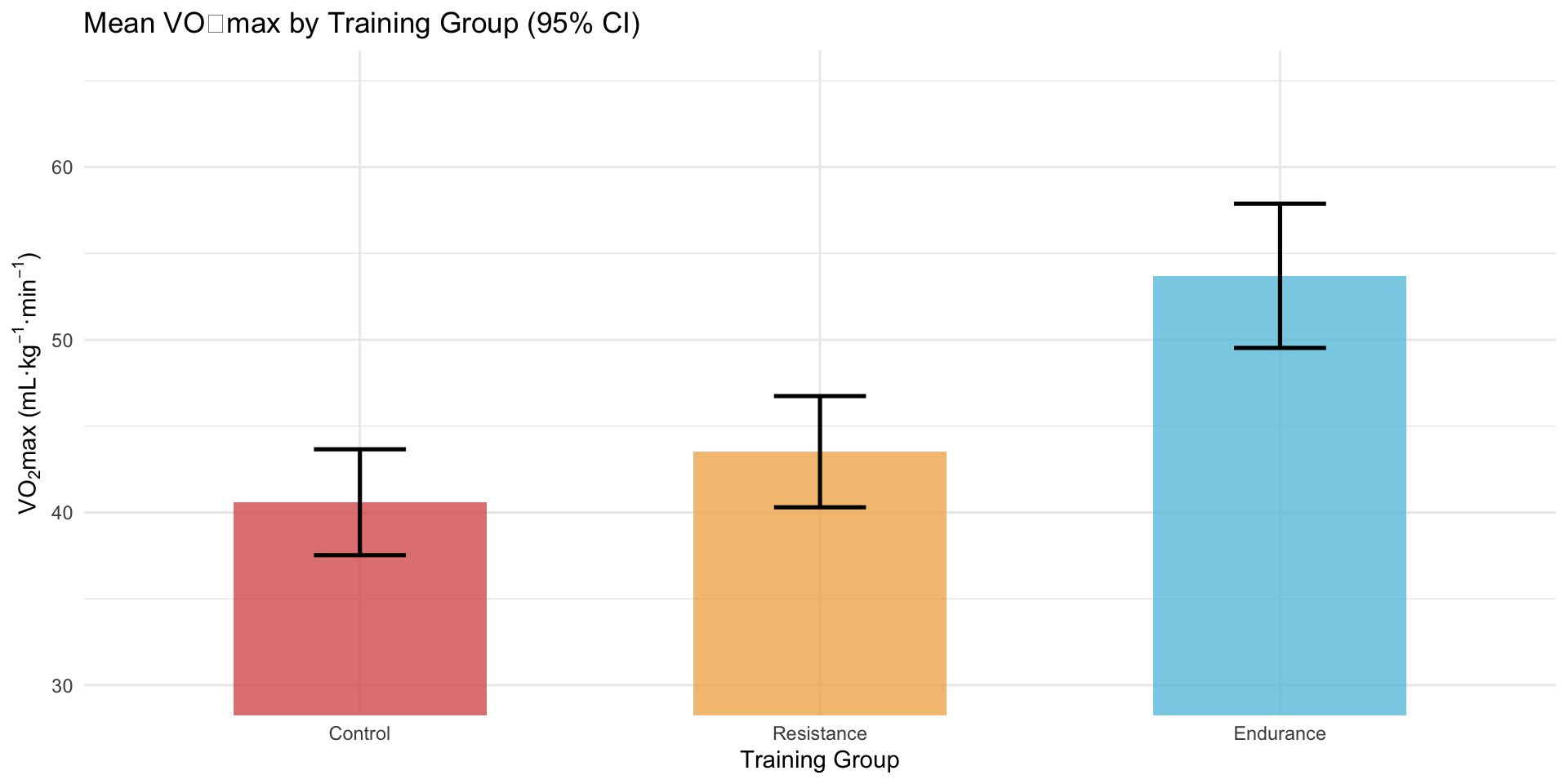
Reading CI Error Bars

Clear gap between two groups’ bars → strong visual evidence of a significant difference. Bars overlap → ambiguous — CIs can overlap by up to ~50% and the difference can still be significant. Always run the formal test; the chart is a guide, not a decision rule.

• Box plots reveal the full distribution: median, IQR, outliers. Good for spotting non-normality.
• Error bar plots with 95% CIs: non-overlapping CIs between endurance and control suggest strong evidence of a difference.
• Overlapping CIs do NOT rule out significance — always run the formal test.

Workflow Summary

Use this sequence whenever you compare means across three or more independent groups^[2,4]:

1. Identify the design — One factor, 3+ independent groups → One-Way ANOVA

2. State hypotheses — H₀: all μ equal; H₁: at least one μ differs

3. Screen your data — Histograms, Q-Q plots, boxplots per group

4. Check assumptions — Shapiro-Wilk (normality), Levene’s test (homogeneity)

5. Run ANOVA in SPSS — Analyze → Compare Means → One-Way ANOVA

6. Interpret omnibus F — Significant? → proceed to post hoc tests

7. Run post hoc tests — Tukey HSD (equal variances) or Games-Howell (unequal)

8. Compute effect sizes — η² = SS_B / SS_T; report ω² as primary

9. Report in APA format — F(df_B, df_W), p, η²/ω², M, SD per group, post hoc results

The Goal Is Not Just Numbers

Always ask: “Is the effect detectable (F, p)? Which groups drive it (post hoc)? How large is it (η², ω²)? Does it matter in practice?”

Reporting One-Way ANOVA in APA Style

APA-style reporting includes: group descriptive statistics, omnibus F, degrees of freedom, p, effect sizes (both η² and ω²), and post hoc comparisons^[17,18]. See the SMS Appendix: APA Reporting for full guidelines.

Omnibus F template:

“A one-way ANOVA revealed a [significant/non-significant] effect of [factor] on [DV], F([df_B], [df_W]) = [F-value], p = [p-value], η² = [value], ω² = [value].”

Full example (from SMS, Ch.14):

A one-way ANOVA revealed a significant effect of training group on VO₂max, F(2, 57) = 14.87, p < .001, η² = .34, ω² = .32. Post hoc comparisons using Tukey HSD indicated that the endurance group (M = 52.4, SD = 6.8 mL·kg⁻¹·min⁻¹) had significantly higher VO₂max than both the resistance group (M = 45.2, SD = 6.2), p = .003, 95% CI [2.1, 12.3], and the control group (M = 40.6, SD = 6.4), p < .001, 95% CI [6.7, 16.9]. Resistance and control groups did not differ significantly, p = .082, 95% CI [−0.5, 9.7].

Key reporting checklist

Include: M and SD per group • F(df_B, df_W) • exact p • η² and ω² • post hoc test name • pairwise p-values and 95% CIs. See the SPSS Tutorial: One-Way ANOVA for full write-up examples.

• Report both η² and ω²: η² for comparability with prior literature; ω² as the less biased estimate.
• Always include group M and SD so readers can judge practical importance of differences.
• CIs around post hoc differences are essential — they show the real-world magnitude.

Sample Size and Power for ANOVA

Statistical power in one-way ANOVA depends on effect size (Cohen’s f), sample size, α, and the number of groups^[12,19].

G*Power: the standard tool

1. Open G*Power
2. Test family: F tests
3. Statistical test: ANOVA: Fixed effects, omnibus, one-way
4. Analysis type: A priori (for sample size planning)
5. Inputs required:
   • Cohen’s f (convert from η²: \(f = \sqrt{\eta^2 / (1-\eta^2)}\))
   • α level (typically .05)
   • Target power (typically .80)
   • Number of groups (\(k\))

Example: Medium effect (f = .25), 80% power, α = .05, 3 groups → ≈ 159 total participants (~53 per group)^[12,19].

Converting η² to Cohen’s f:

η²	f	Interpretation
.01	.10	Small
.06	.25	Medium
.14	.40	Large
.34	.72	Very large

SPSS Power Analysis

SPSS Statistics 31+ includes built-in power analysis: Analyze → Power Analysis → One-Way ANOVA. Useful for both a priori (planning) and post hoc (achieved power) analyses.

• Base effect size estimates on pilot data or the smallest effect that would matter in practice — not just “medium.”
• Each additional group requires more participants for the same power, even if effect size is constant.
• Power < .80 means the study will frequently miss real effects (false negatives).

Common Pitfalls

Avoid these frequent mistakes when conducting and reporting one-way ANOVA^[1,2,15]:

#	Pitfall	Solution
1	Running multiple t-tests instead of ANOVA	Always use ANOVA as the omnibus test; post hoc tests for pairwise follow-up
2	Running post hoc tests after a non-significant F	Post hoc tests are only valid after a significant omnibus result
3	Reporting η² without acknowledging its bias	Report ω² as primary; note η²’s upward bias when including it
4	Treating non-significant F as proof of no difference	A non-significant result ≠ groups are equal; may reflect low power
5	Ignoring unequal group sizes	Aim for balanced designs; report group-specific descriptives

Pitfall 4 explained

Failing to reject H₀ does not establish that group means are equal — it only means the evidence was insufficient to detect a difference^[20,21]. A non-significant result with a wide CI and moderate ω² may simply indicate an underpowered study, not the absence of a real effect.

• Pitfall 2 is surprisingly common in student lab reports — reinforce the “omnibus F first” rule.
• Pitfall 3: when comparing to older literature that reports only η², report both and flag the difference.
• Pitfall 4: “absence of evidence is not evidence of absence” — requires adequate power to support a null result.

Key Takeaways

1. ANOVA is required when comparing three or more group means—multiple t-tests inflate the familywise error rate unacceptably.
2. Variance partitioning: \(SS_{\text{total}} = SS_{\text{between}} + SS_{\text{within}}\). The F-ratio is the signal (\(MS_B\)) divided by the noise (\(MS_W\)).
3. F ≈ 1 when H₀ is true; F > 1 when group means truly differ. The larger the F, the stronger the evidence against H₀.
4. Assumptions matter: Check independence (design), normality (Shapiro-Wilk per group), and homogeneity of variance (Levene’s test). Violations have specific remedies.
5. Post hoc tests are only appropriate after a significant omnibus F. Use Tukey HSD when variances are equal; Games-Howell when they are not.
6. Effect sizes: Report ω² (preferred) alongside η². Cohen’s benchmarks: small = .01, medium = .06, large = .14.
7. Statistical significance ≠ practical significance. Always interpret the effect size alongside the p-value.
8. Visualize first: Box plots and mean-CI plots across groups reveal distributional shapes and suggest where differences lie before formal testing.

Core Principle

Always ask: “Are the groups different (F, p)? Which ones (post hoc)? How much (η², ω²)? Does it matter in practice?”

Practice Questions

1. A researcher compares injury rates across four sports (soccer, basketball, swimming, tennis) using a continuous injury severity score. Which test is appropriate and why?
2. SPSS output shows: F(3, 76) = 6.43, p = .001, Levene’s F = 1.12, p = .347. State your conclusion and the appropriate post hoc test to use.
3. From an ANOVA source table: \(SS_B = 480\), \(SS_W = 1,560\), \(k = 4\), \(N = 64\). Compute \(df_B\), \(df_W\), \(MS_B\), \(MS_W\), and \(F\).
4. Why is \(\omega^2\) preferred over \(\eta^2\) when reporting ANOVA effect sizes?
5. A researcher obtains F(2, 57) = 2.41, p = .098. Should post hoc tests be conducted? Explain.
6. Tukey HSD output shows a mean difference of 8.3 with a 95% CI of [−0.2, 16.8]. Is this comparison statistically significant? What does the CI suggest about practical significance?
7. A one-way ANOVA yields η² = .08. Interpret this using Cohen’s benchmarks and explain what it means in plain language.
8. Explain in your own words why the F-ratio is approximately 1 when the null hypothesis is true.
9. A researcher has four groups with n = 10, 10, 10, 12. Levene’s test is p = .041. What should the researcher do, and which post hoc test should be used?

Exit Ticket: One-Way ANOVA Activity

Your instructor will provide you with a link to the activity in Canvas

References

1. Maxwell, S. E., Delaney, H. D., & Kelley, K. (2018). Designing experiments and analyzing data: A model comparison perspective (3rd ed.). Routledge.

2. Field, A. (2018). Discovering statistics using IBM SPSS statistics (5th ed.). SAGE Publications.

3. Fisher, R. A. (1925). Statistical methods for research workers.

4. Moore, D. S., McCabe, G. P., & Craig, B. A. (2021). Introduction to the practice of statistics (10th ed.). W. H. Freeman; Company.

5. Vincent, W. J. (2005). Statistics in kinesiology.

6. Thomas, L. (2015). How to estimate power and sample size. Trauma Surgery & Acute Care Open, 1(1), e000005. https://doi.org/10.1136/tsaco-2015-000005

7. Portney, L. G., & Watkins, M. P. (2020). Foundations of clinical research: Applications to practice.

8. Blanca, M. J., Alarcón, R., Arnau, J., Bono, R., & Bendayan, R. (2013). Non-normal data: Is ANOVA still a valid option? Psicothema, 25(4), 552–557. https://doi.org/10.7334/psicothema2013.552

9. Levene, H. (1960). Robust tests for equality of variances. Contributions to Probability and Statistics: Essays in Honor of Harold Hotelling, 278–292.

10. Games, P. A., & Howell, J. F. (1976). Pairwise multiple comparison procedures with unequal n’s and/or variances: A monte carlo study. Journal of Educational Statistics, 1(2), 113–125. https://doi.org/10.3102/10769986001002113

11. Tukey, J. W. (1949). Comparing individual means in the analysis of variance. Biometrics, 5(2), 99–114. https://doi.org/10.2307/3001913

12. Cohen, J. (1988). Statistical power analysis for the behavioral sciences (2nd ed.). Lawrence Erlbaum Associates.

13. Lakens, D. (2013). Calculating and reporting effect sizes to facilitate cumulative science: A practical primer for t-tests and ANOVAs. Frontiers in Psychology, 4, 863. https://doi.org/10.3389/fpsyg.2013.00863

14. Cumming, G. (2014). The new statistics: Why and how. Psychological Science, 25(1), 7–29. https://doi.org/10.1177/0956797613504966

15. Olejnik, S., & Algina, J. (2003). Generalized eta and omega squared statistics: Measures of effect size for some common research designs. Psychological Methods, 8(4), 434–447. https://doi.org/10.1037/1082-989X.8.4.434

16. Cumming, G. (2012). Understanding the new statistics: Effect sizes, confidence intervals, and meta-analysis. Routledge.

17. Wilkinson, L., & Task Force on Statistical Inference. (1999). Statistical methods in psychology journals: Guidelines and explanations. American Psychologist, 54(8), 594–604. https://doi.org/10.1037/0003-066X.54.8.594

18. American Psychological Association. (2020). Publication manual of the american psychological association (7th ed.). American Psychological Association.

19. Faul, F., Erdfelder, E., Lang, A.-G., & Buchner, A. (2007). G*power 3: A flexible statistical power analysis program for the social, behavioral, and biomedical sciences. Behavior Research Methods, 39(2), 175–191. https://doi.org/10.3758/BF03193146

20. Altman, D. G., & Bland, J. M. (1995). Statistics notes: Absence of evidence is not evidence of absence. BMJ, 311, 485. https://doi.org/10.1136/bmj.311.7003.485

21. Cohen, J. (1994). The earth is round (p < .05). American Psychologist, 49(12), 997–1003. https://doi.org/10.1037/0003-066X.49.12.997

22. Furtado, O., Jr. (2026). Statistics for movement science: A hands-on guide with SPSS (1st ed.). https://drfurtado.github.io/sms/