Week 5: Descriptive Statistics

KIN 610 - Spring 2023

Dr. Ovande Furtado Jr

Credits

(furtadoDescriptiveStatistics2023?)

Descriptive Stats

• Measures of central tendency
• Measures of variability
• Tables and graphs

Symbols

Measure	Symbol
Mean (population)	\(\mu\)
Mean (sample)	\(\bar{x}\)
Median	\(med\)
Mode	\(mode\)
Range	\(R\)
Interquartile Range	\(IQR\)
Variance (population)	\(\sigma^2\)
Variance (sample)	\(s^2\)
Standard Deviation (population)	\(\sigma\)
Standard Deviation (sample)	\(s\)

Measures of Central Tendency

The Mean

• The mean is the most commonly used measure of central tendency in Kinesiology research.
• It is the arithmetic average of a data set.
• Calculated by adding up all the values and dividing by the total number of values.

Why Mean?

• The mean considers all the values in a data set.
• Sensitive to small changes in the data.
• Appropriate for continuous (normal) data

Limitations of Mean

• Not always the most appropriate measure of central tendency.
• Extreme outliers or skewed data can influence the mean.

library(stats)

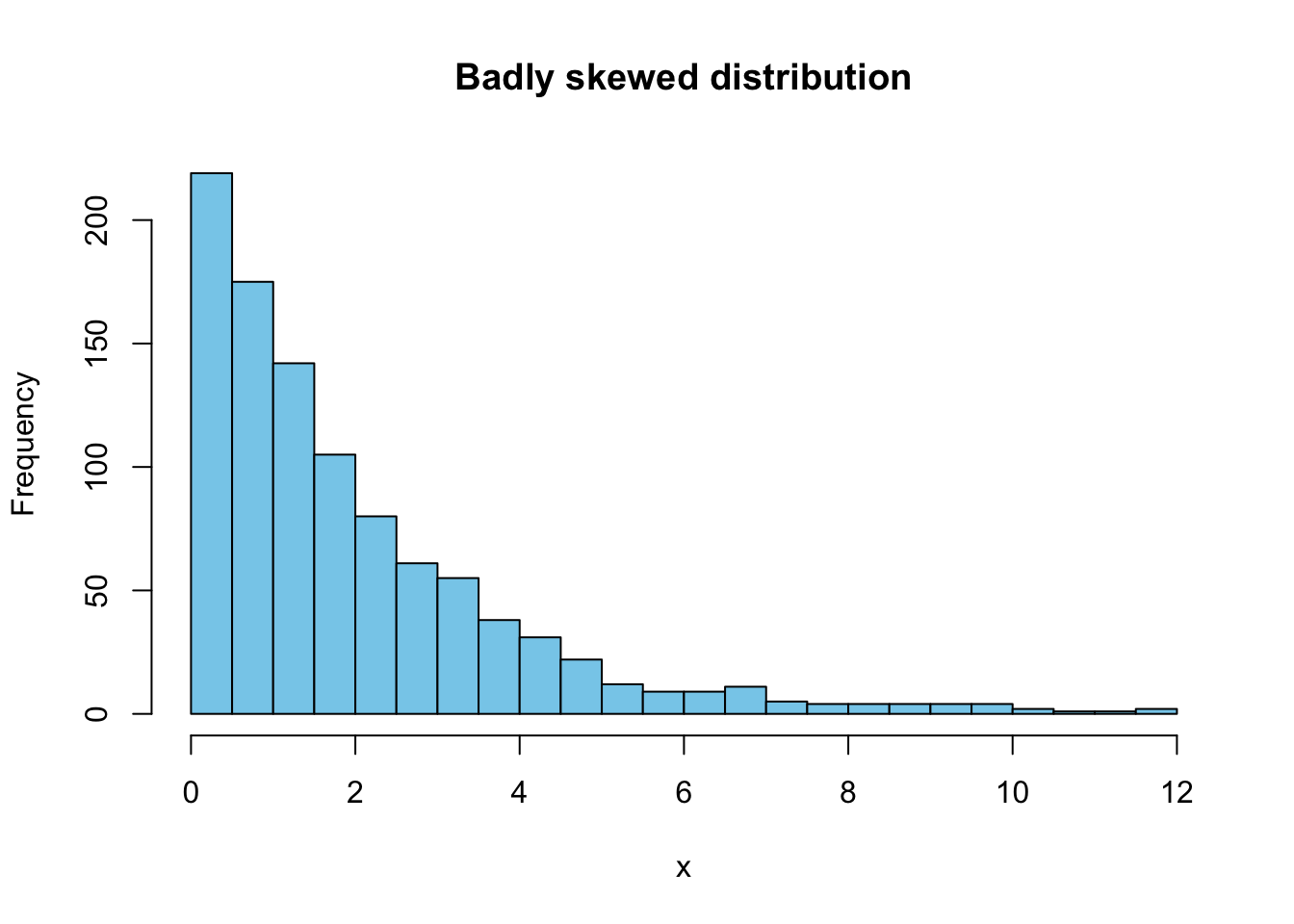
# Generate a gamma distributed random variable
x <- rgamma(n = 1000, shape = 2, rate = 1)

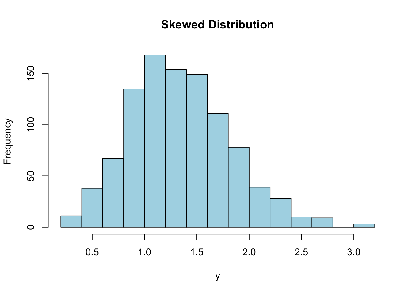
# Create a skewed distribution by taking the square root of the gamma variable
y <- sqrt(x)

# Plot the histogram of the skewed distribution
hist(y, breaks = 20, col = "lightblue", main = "Skewed Distribution")

Median as an alternative

• If data are continuous but deviating from normality
• The median is not as sensitive to extreme values as the mean.
• Appropriate with skewed data or data with outliers.

set.seed(123)  # for reproducibility

# Generate 1000 samples from a chi-squared distribution with 2 degrees of freedom
x <- rchisq(1000, df = 2)

# Plot the histogram of x
hist(x, breaks = 20, col = "skyblue", main = "Badly skewed distribution")

Calculating the Mean - Steps

• Add up all the values in the dataset.
• Count the number of observations in the dataset.
• Divide the total sum by the number of observations.

Calculating the Mean - Example

Data set: 12.5, 10.8, 11.2, 13.1, 12.9, 11.7, 12.3

• Step 1: 12.5 + 10.8 + 11.2 + 13.1 + 12.9 + 11.7 + 12.3 = 84.5
• Step 2: 7
• Step 3: 84.5 / 7 = 12.07 seconds

Calculating the Mean - Equation

\[ \bar{x} = \frac{1}{n}\sum_{i=1}^{n}x_i \]

where, \(n\) is the total number of values in the set, \(x_i\) is the \(i\)th value in the set, and \(\sum_{i=1}^{n}\) represents the sum of all the values from \(i=1\) to \(i=n\).

Displaying data¹

library(ggplot2)

# Create a data frame with 3 group means
group_means <- data.frame(group = c("Group 1", "Group 2", "Group 3"),
                          mean = c(10, 15, 12))

# Create a bar chart with custom colors and labels
ggplot(group_means, aes(x = group, y = mean, fill = group)) +
  geom_col() +
  scale_fill_manual(values = c("#FFA07A", "#87CEEB", "#90EE90")) +  # custom colors
  labs(title = "Comparison of Group Means in Kinesiology",
       x = "Groups", y = "Mean Values")

1. Bar chart created in RStudio.

Median

• Definition of Median
• Median is not influenced by extreme values
• Median may not be as sensitive to small changes in the data as the mean
• Both case below the median is 7
• data1: 1, 3, 7, 7, 8, 99
• data2: 1, 3, 7, 7, 8, 9

Median Calculation

• First step is arranging the data in order of magnitude
• Median is the middle value if the number of observations is odd
• Median is the average of two middle values if the number of observations is even
• Use of median when data contains extreme values or is ordinal
• Helps to understand the group’s typical value or performance
• Example in the next slide

Mode

• Definition of Mode
• Mode is the value that occurs most frequently in a data set
• Mode is often used with categorical or nominal data

Mode Calculation

• Identify the value or category that occurs most frequently in the data set
• Helps researchers identify the most common value or category in a data set

Comparison table

Measure of Central Tendency	Definition	Calculation	Usefulness
Mean	The average of a set of numbers	Sum of values divided by number of values	Useful for data that are normally distributed and have no extreme values
Median	The middle value in a set of numbers	Order values and find the middle value	Useful for data with extreme values or that are not normally distributed
Mode	The value that occurs most frequently in a set of numbers	Identify the value that appears most often	Useful for categorical or nominal data

Measures of Variability

Introduction

• Understanding how much individual data points in a data set vary from one another
• Types: variance, standard deviation, range, and interquartile range
• Importance

  • understanding data sets

  • can help researchers understand the precision and accuracy of their results

  • to draw meaningful conclusions

Range

• Difference between the largest and smallest values in a data set
• Limitations of range due to sensitivity to outliers or extreme values
• Caution in interpreting the range especially when there are outliers
• The need to use range in conjunction with other measures of variability

Calculating Range

• Use of jamovi to obtain the minimum and maximum values for a data set
• Calculation of the range by subtracting the minimum from the maximum value

Interquartile Range

• Definition of interquartile range as a measure of variability that is less sensitive to outliers
• Use of quartiles to divide a data set into four equal parts
• Calculation of interquartile range as the difference between the upper and lower quartiles
• Importance of interquartile range in providing information about the range of the middle 50% of the data

Calculating Interquartile Range

• Calculation: Q3 - Q1
• Interpretation: the range between the first quartile and the third quartile
• Advantages: Resistant to outliers
• Disadvantages: Not sensitive to extreme values that fall outside the range of the interquartile

Variance

\(s^2 = \frac{\sum_{i=1}^{n}(x_i-\bar{x})^2}{n-1}\)

• Interpretation: A measure of how much the data deviates from the mean
• Advantages: Widely used and well known
• Disadvantages: Can be sensitive to outliers

Standard Deviation

• Calculation: \(s = \sqrt{\frac{\sum_{i=1}^{n}(x_i - \bar{x})^2}{n-1}}\)
• Interpretation: A measure of the amount of variation or dispersion of a set of values from the mean
• Advantages: Widely used and well known
• Disadvantages: Can be sensitive to outliers; more difficult to interpret than the range or IQR

Coefficient of Variation

• Calculation: CV = \(\frac{s}{\bar{x}} \times 100%\)
• Interpretation: A measure of the relative variation or dispersion of a data set, particularly useful for comparing the variability of data sets with different units or scales
• Advantages: Allows for comparison of the relative variability of data sets with different scales or units
• Disadvantages: Not suitable for data sets with negative or zero mean values

Comparing Measures of Variability

• It is essential to consider the characteristics of the data and the research question when comparing measures of variability.
• Range and IQR are useful for non-normally distributed data or when identifying outliers.
• Variance and standard deviation are useful for normally distributed data and can provide more information about the spread of the distribution.
• Coefficient of variation is suitable for comparing the spread of two sets of data with different units.

Comparison table

Measure of Variability	Calculation	Interpretation	Advantages	Disadvantages
Range	Maximum value - Minimum value	The spread of the data from the smallest to the largest value	Easy to understand	Sensitive to outliers
Interquartile Range	Q3 - Q1	The range between the first quartile and the third quartile	Resistant to outliers	Not sensitive to extreme values that fall outside the range of the interquartile
Variance	\(s^2 = \frac{\sum_{i=1}^{n}(x_i-\bar{x})^2}{n-1}\)	A measure of how much the data deviates from the mean	Widely used and well known	Can be sensitive to outliers
Standard Deviation	\(s = \sqrt{\frac{\sum_{i=1}^{n}(x_i - \bar{x})^2}{n-1}}\)	A measure of the amount of variation or dispersion of a set of values from the mean	Widely used and well known	Can be sensitive to outliers; more difficult to interpret than the range or IQR

Using jamovi

• Open jamovi, click Exploration, then Descriptives
• Move DVs under Variables and IVs under Split by
• Select Variables across rows under Descriptives (horizontal format)
• jamovi will create a Descriptives Table - see next slide.

Descriptives Table

Summary

• Descriptive statistics help in summarizing and describing a dataset’s features.
• Measures of variability are used to understand how spread out the data is.
• The range, interquartile range, variance, standard deviation, and coefficient of variation are measures of variability that have their advantages and disadvantages.
• The choice of measure depends on the characteristics of the data and the research question.

Practice Exercises

Find several exercises by clicking here

References